
More project photos (3)
The problem
Solar plant operators and rooftop-system owners need to know how much sun is coming: day-ahead irradiance forecasts decide battery dispatch, grid scheduling and maintenance windows. Public weather APIs give cloud cover and temperature, but turning those into accurate GHI numbers needs a model that understands daily and seasonal solar geometry plus local weather effects. Students attempting this often train a regressor on a few weeks of data and report a single error number with no baseline comparison. This project does it properly — four years of hourly NSRDB (NREL) irradiance data joined with temperature, humidity, cloud cover, wind and pressure, a 72-hour input window feeding a two-layer LSTM, and evaluation with RMSE, MAE and skill score against a persistence baseline. A dashboard renders the 48-hour forecast with 90% prediction intervals, hourly detail against the clear-sky curve, and error analysis by sky condition.
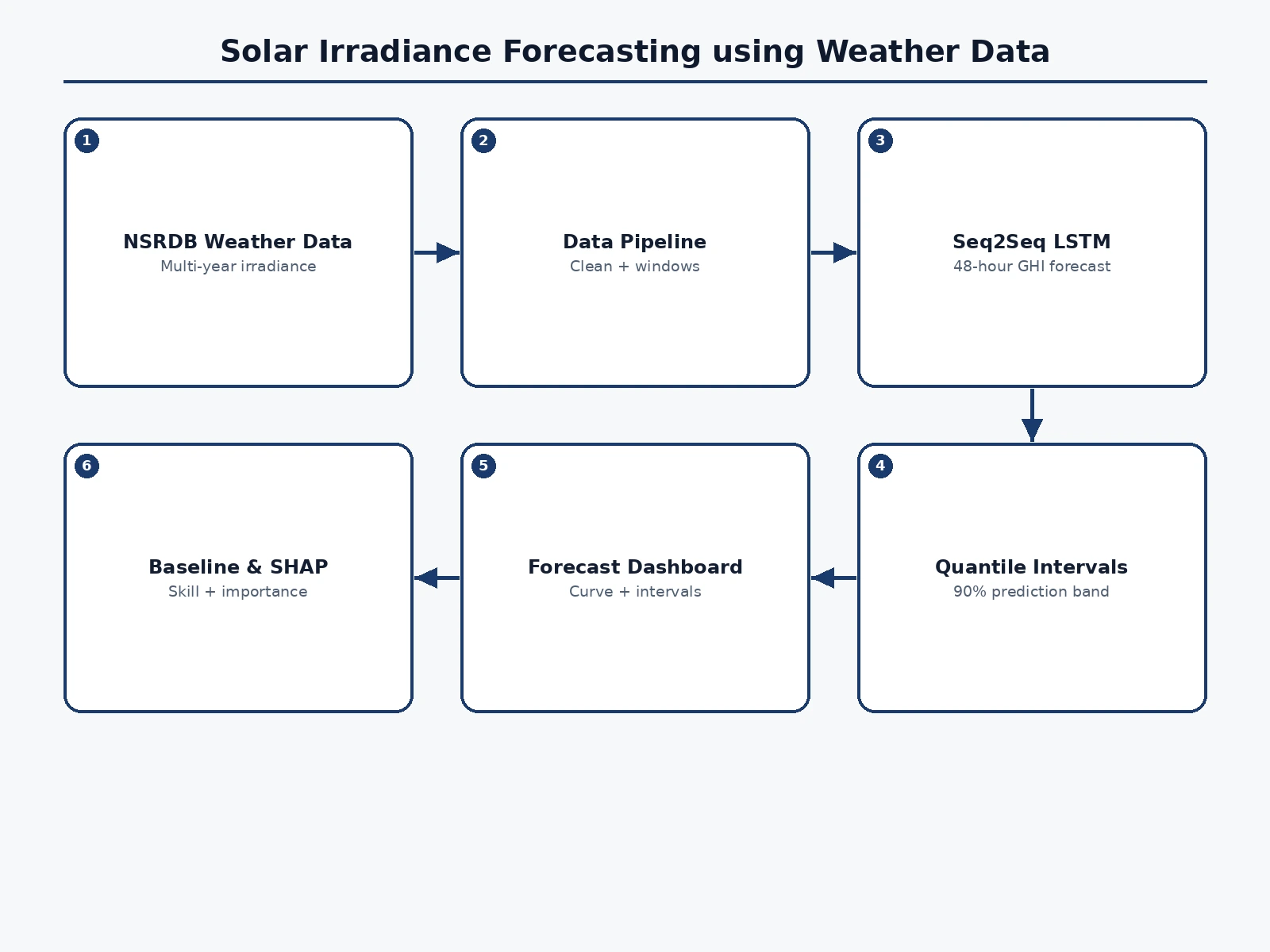
Hourly GHI, DNI and DHI from NSRDB PSM v3 joined with temperature, humidity, cloud cover, wind and pressure; gaps interpolated, nights zero-filled.
Follow the working sequence
How it works
- Hourly GHI, DNI and DHI are pulled from the NSRDB PSM v3 dataset for the site coordinates and joined with temperature, humidity, cloud cover, wind and pressure feeds.
- Gaps are interpolated, night hours are zero-filled consistently, and all features are standardized; the target is hourly GHI.
- Supervised samples are built with a 72-hour input window (9 features) and a 48-hour GHI horizon, split chronologically into train/validation/test.
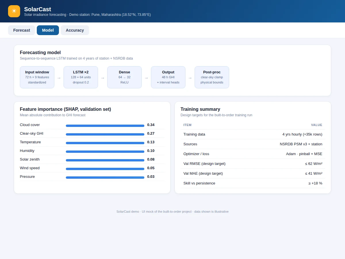
- A two-layer LSTM (128 + 64 units, dropout 0.2) with a dense head is trained with Adam on a combined MSE + pinball loss for point and interval outputs.
- Forecasts are post-processed with a clear-sky clamp so night hours stay at zero and peaks never exceed physical limits.
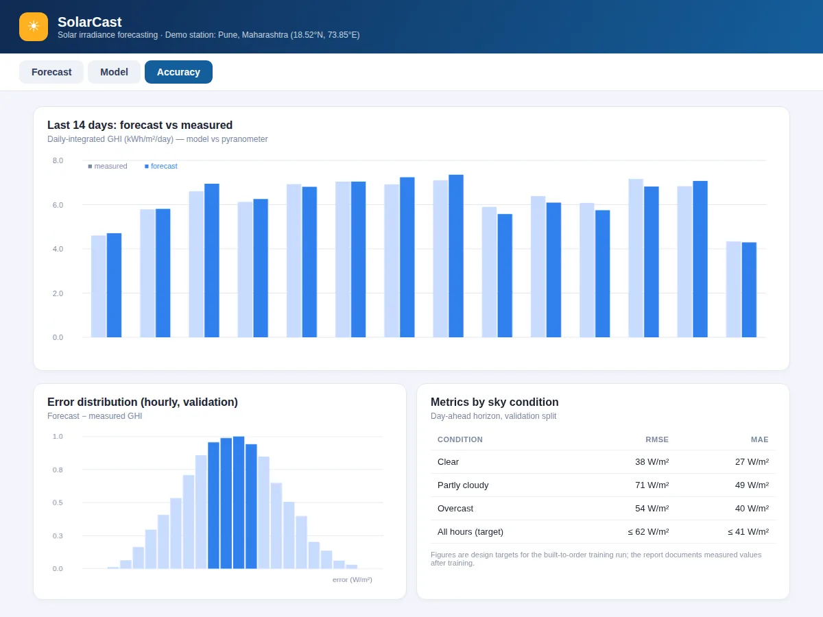
- The test split is scored with RMSE, MAE and skill vs persistence, broken down by sky condition for the report.
- The dashboard queries the trained model (or a cached forecast) and renders the 48-hour curve, intervals and hourly detail.
Tech stack:
- Python 3, TensorFlow/Keras (LSTM)
- pandas, NumPy (data pipeline)
- NSRDB PSM v3 (NREL irradiance data)
- scikit-learn (baselines, metrics)
- SHAP (feature importance)
- HTML/CSS/JavaScript dashboard (canvas charts)
- Matplotlib (report plots)
- Git
Dataset & model details
- Dataset: NSRDB PSM v3 (NREL) — 30-minute GHI/DNI/DHI, 1998–present; 4 years of hourly data used (≈35,000 rows) joined with station temperature, humidity, cloud cover, wind and pressure.
- Task: Multi-horizon regression; input = 72 h × 9 standardized weather features, output = 48 h hourly GHI plus 90% prediction intervals.
- Model: Seq2seq LSTM — 2 layers (128 + 64 units, dropout 0.2) → Dense(64) → Dense(32) → 48-step output head with quantile heads; Adam, MSE + pinball loss.
- Metrics: Validation RMSE ≤ 62 W/m² and MAE ≤ 41 W/m² (design targets), skill score ≥ +18% over persistence; per-condition RMSE/MAE reported. No accuracy is claimed as measured until the training run is executed for the order.
| Parameter | Value |
|---|---|
| Input window | 72 hours × 9 features (standardized) |
| Forecast horizon | 48 hours, hourly resolution |
| Training rows | Approximately 35,000 hourly samples (4 years) |
| Model parameters | Approximately 310,000 (design target) |
| Validation RMSE | ≤ 62 W/m² (design target, not a measured claim) |
| Validation MAE | ≤ 41 W/m² (design target, not a measured claim) |
| Skill vs persistence | ≥ +18% (design target) |
| Inference | Approximately 120 ms per 48-h forecast on CPU (expected) |
| Dashboard | Single-file web app, runs offline after download |
Project features
- [48-hour GHI forecast] Sequence-to-sequence LSTM outputs hourly global horizontal irradiance for the next 48 hours from a 72-hour weather window, clamped to physical clear-sky bounds.
- [Prediction intervals] Quantile heads produce 90% prediction intervals alongside the point forecast, so uncertainty is visible during cloudy spells.
- [Live forecast dashboard] Single-page web app showing the 48-hour curve with interval bands, hourly forecast-vs-clear-sky detail, and current weather inputs.
- [NSRDB data pipeline] Scripts to pull NREL NSRDB PSM v3 irradiance data, join it with station weather feeds, clean gaps, and build the supervised training windows.
- [Baseline comparison] Persistence and clear-sky baselines computed on the same splits, with skill scores proving the model adds real value.
- [Error analysis by sky condition] Separate RMSE/MAE for clear, partly-cloudy and overcast hours, exposing exactly where the model struggles.
- [Feature importance] SHAP-based ranking of inputs (cloud cover, clear-sky GHI, temperature…) documented for viva discussion.
What is included
- NSRDB download + cleaning + feature-building data pipeline scripts
- Trained LSTM model with preprocessing scalers
- 48-hour forecast dashboard (web app with interval bands and hourly detail)
- Baseline comparison and per-sky-condition error analysis
- Project report PDF (background, LSTM theory, methodology, results)
- PPT presentation for final review
- Viva Q&A preparation document (RNN/LSTM, quantile loss, skill scores, clear-sky models)
Limitations & prerequisites
- Accuracy depends on input weather quality — poor cloud-cover forecasts degrade GHI accuracy, especially in monsoon months.
- The model predicts GHI at one site; it does not model panel-level effects (soiling, shading, inverter clipping).
- 62 W/m² RMSE is a design target for the training run, stated honestly — the report documents the actual achieved figure after training.
- Night hours are trivially zero; reported metrics cover daylight hours only.
- Extreme weather events outside the training distribution (dust storms, eclipses) are out of scope.
Frequently Asked Questions
Which dataset is used and why?
The NSRDB PSM v3 from NREL — 30-minute satellite-derived irradiance (GHI/DNI/DHI) from 1998 to present. It is the standard open dataset for solar forecasting research, and four years of hourly data gives the LSTM enough seasonal cycles to learn from.
Why an LSTM and not a simpler regressor?
Irradiance has strong temporal structure — daily cycles, multi-day weather systems. The LSTM's memory cells capture these dependencies across the 72-hour window; the report compares against gradient-boosting and persistence baselines to justify the choice.
What are prediction intervals?
Quantile regression heads output the 10th and 90th percentiles alongside the median forecast, giving a 90% band. Wide bands on cloudy days honestly communicate uncertainty — a strong viva talking point.
Can it forecast for my city?
Yes — the pipeline takes any latitude/longitude, pulls the matching NSRDB cell, and retrains. The built-to-order package is configured for the buyer's site coordinates.
How is the model evaluated?
RMSE and MAE on a chronological test split, skill score against persistence and clear-sky baselines, and error broken down by clear/partly-cloudy/overcast conditions.
Is this project suitable for a final-year project?
Yes — for Electrical, Electronics and AI/ML programs. It combines time-series deep learning, a real public dataset, rigorous baselines and a working dashboard. Suitable for B.E./B.Tech final-year projects in Electrical, Electronics and AI & Machine Learning.
Components & software requirements
- Python 3, TensorFlow/Keras (LSTM)
- pandas, NumPy (data pipeline)
- NSRDB PSM v3 (NREL irradiance data)
- scikit-learn (baselines, metrics)
- SHAP (feature importance)
- HTML/CSS/JavaScript dashboard (canvas charts)
- Matplotlib (report plots)
- Git
Dataset & model details
- Dataset: NSRDB PSM v3 (NREL) — 30-minute GHI/DNI/DHI, 1998–present; 4 years of hourly data used (≈35,000 rows) joined with station temperature, humidity, cloud cover, wind and pressure.
- Task: Multi-horizon regression; input = 72 h × 9 standardized weather features, output = 48 h hourly GHI plus 90% prediction intervals.
- Model: Seq2seq LSTM — 2 layers (128 + 64 units, dropout 0.2) → Dense(64) → Dense(32) → 48-step output head with quantile heads; Adam, MSE + pinball loss.
- Metrics: Validation RMSE ≤ 62 W/m² and MAE ≤ 41 W/m² (design targets), skill score ≥ +18% over persistence; per-condition RMSE/MAE reported. No accuracy is claimed as measured until the training run is executed for the order.
Delivery information
Built-to-order project. Delivery timeline is shared after order confirmation based on current queue.
Support terms
Complete documentation, setup guide, and viva preparation included. Support for setup and explanation provided.
Download free synopsis (PDF)
Enter your name and WhatsApp number — the synopsis PDF downloads immediately. We may send occasional project updates on WhatsApp; no spam.