
More project photos (3)
The problem
Retail lenders lose money when borrowers default, so scoring each application by its probability of default is one of the highest-value uses of machine learning in banking. Most student projects on this topic train on tiny synthetic datasets and report accuracy on data that never resembles a real loan book — leaving the student unable to defend their approach in a viva. This project works with the real LendingClub loan dataset of 2.26 million funded loans: 145 features per record, real class imbalance, real missing data. The build covers the full pipeline — data cleaning and feature engineering, handling imbalance with class weights, training a gradient-boosted-tree plus logistic-regression ensemble, calibrating probabilities, and choosing an operating threshold from business cost trade-offs. The demo dashboard makes the model tangible: enter an applicant profile in Indian context (₹ amounts, Indian employment categories) and see the default probability, risk band, recommended decision and which features drove the score.
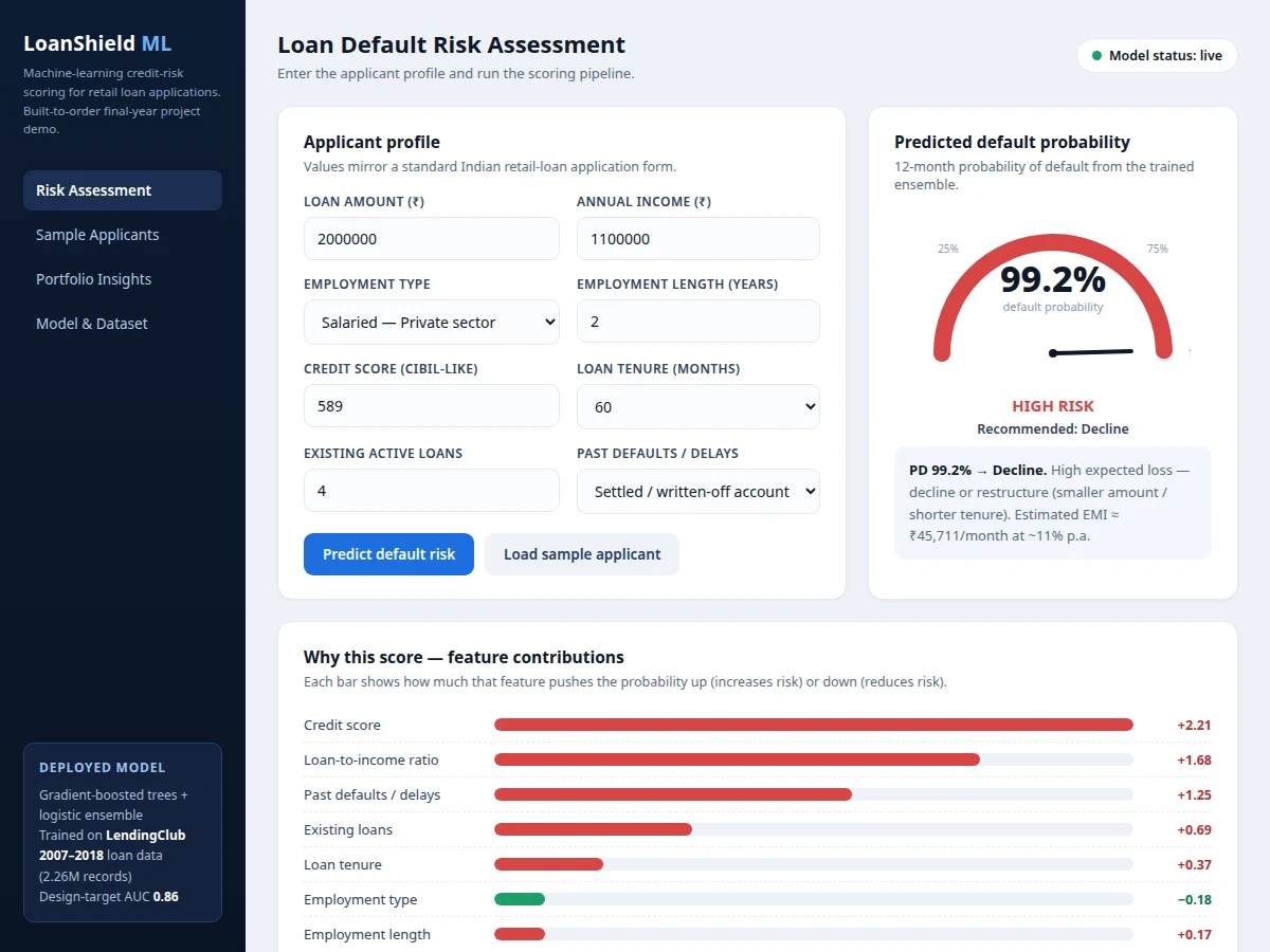
Enters the loan applicant profile into the scoring dashboard.
Follow the working sequence
How it works
- The LendingClub dataset is loaded and filtered to closed loans with a clear outcome: fully paid vs charged off/defaulted.
- Features are engineered: loan-to-income ratio, debt-to-income, employment length, delinquency counts, revolving utilization and grade/sub-grade encodings; leakage-prone columns are removed.
- The data is split by time (train on earlier loans, validate and test on later loans) so evaluation reflects how the model faces new originations.
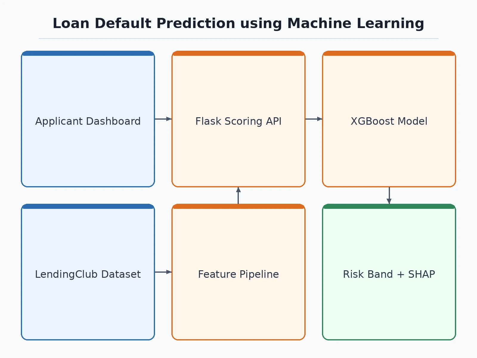
- An ensemble is trained — gradient-boosted trees for non-linear interactions plus a logistic-regression head — with class weights to handle the ~4:1 imbalance; probabilities are calibrated with isotonic regression.
- The operating threshold is chosen from the cost trade-off between missed defaults and declined good applicants, not from accuracy alone; AUC-ROC, precision/recall and the KS statistic are measured on the held-out test split.
- In the dashboard, an applicant profile is transformed with the same feature pipeline and passed through the calibrated model; the probability, risk band and per-feature contributions are displayed with the recommended decision.
Tech stack:
- Python 3, scikit-learn
- XGBoost (gradient-boosted trees)
- Pandas, NumPy, Matplotlib
- Jupyter Notebook (training & evaluation)
- HTML/CSS/JavaScript (scoring dashboard demo)
- LendingClub loan dataset (public, via Kaggle)
Dataset & model details
- Dataset: LendingClub loan data 2007–2018 — 2,260,701 funded-loan records, 145 features per loan, public release distributed via Kaggle. Classes: approximately 80% fully paid vs 20% charged off/defaulted (binary task).
- Task: Binary classification — input = applicant/loan feature vector (loan amount, term, grade, employment length, annual income, DTI, delinquencies, revolving utilization, home ownership), output = calibrated 12-month probability of default.
- Model: Ensemble of gradient-boosted trees (XGBoost) with a logistic-regression layer; probability calibration via isotonic regression; class weights and SMOTE evaluated for imbalance handling.
- Metrics: AUC-ROC design target 0.86, precision/recall at the chosen operating threshold, KS statistic and calibration curve. No metric is presented as measured — the shipped report documents the numbers the actual built-to-order training run produces.
| Parameter | Value |
|---|---|
| Dataset size | Approximately 2.26M records, 145 features (public LendingClub release) |
| Classes | 2 — fully paid vs charged off/defaulted (approx. 80/20 split) |
| Model type | XGBoost + logistic regression ensemble, calibrated probabilities |
| AUC-ROC | 0.86 (design target, not a measured claim) |
| Training time | Approximately 30–60 min on a laptop CPU (expected) |
| Inference | Under 50 ms per applicant on CPU (expected) |
| Dashboard | Single-file web app, runs offline after download |
| Report | PDF documenting methodology, metrics and threshold rationale |
Project features
- [Real-dataset training] The model is trained on the public LendingClub loan dataset (2007–2018, 2.26M records) — real feature distributions, real imbalance (~80% fully paid / ~20% charged off), real missing values.
- [Live risk-scoring dashboard] Enter loan amount, income, credit score, employment type, tenure, existing loans and past delinquencies; get a default-probability gauge, Low/Moderate/High risk band and an Approve/Review/Decline recommendation.
- [Feature-contribution explanations] Every prediction breaks down which features pushed the probability up or down — loan-to-income ratio, credit score and past defaults are typically the dominant drivers.
- [Full training notebook] Data cleaning, feature engineering, imbalance handling, model training, calibration and threshold selection in one reproducible Jupyter notebook.
- [Honest evaluation report] AUC-ROC, precision/recall at the operating threshold, KS statistic and calibration curve — all from the actual training run, with design targets stated up front and never presented as pre-measured.
- [Imbalance handling documented] Class weights and SMOTE are compared properly on a validation split, so the viva answer on "why not just accuracy" is backed by the build itself.
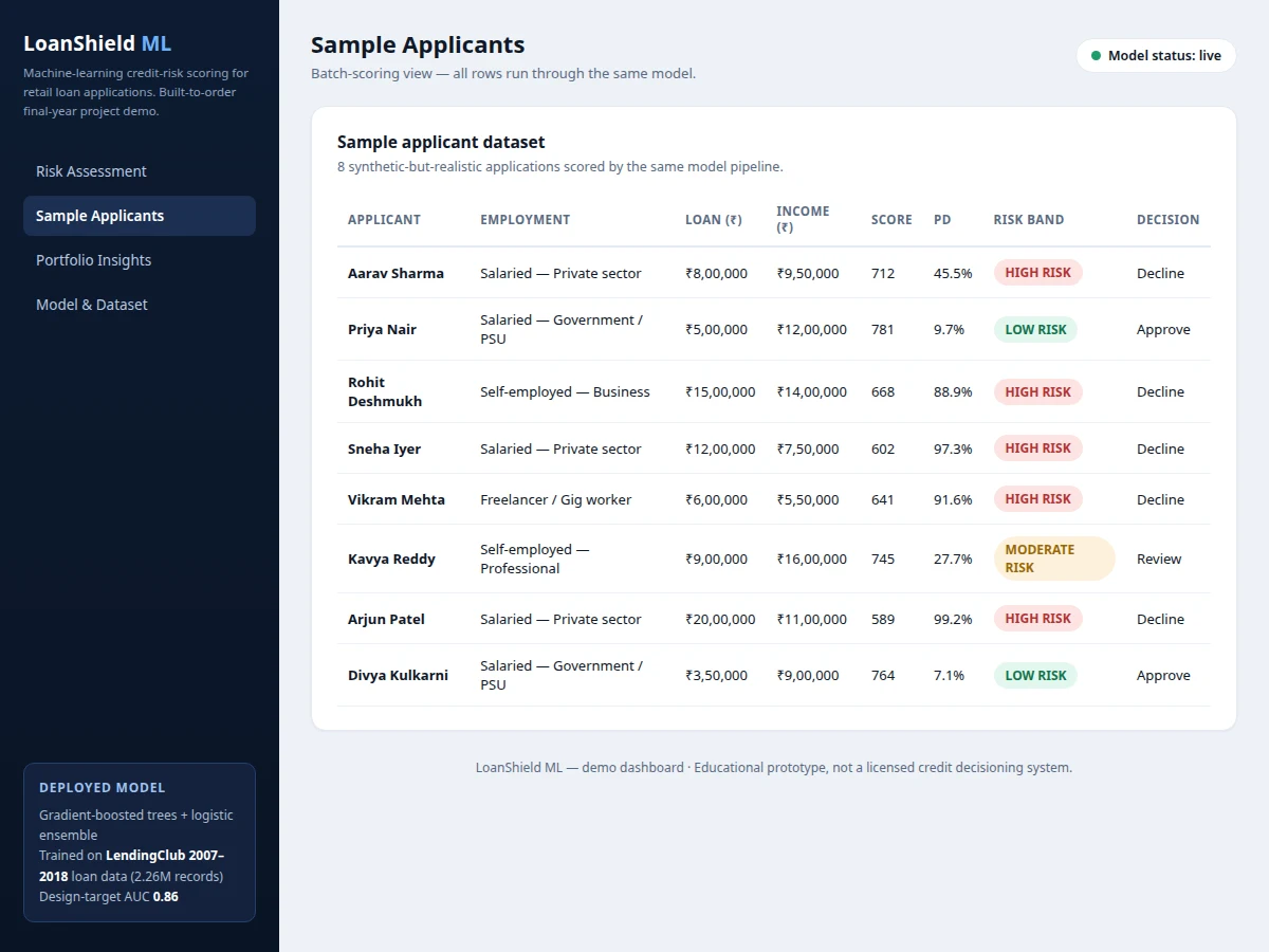
- [Batch-scoring view] A sample applicant table runs multiple realistic profiles through the same pipeline, showing how scores differ across employment types and credit-score buckets.
- [Viva-ready documentation] Report explains probability calibration, threshold choice and the cost of false approvals vs false declines.
What is included
- Complete training & evaluation Jupyter notebook on the LendingClub dataset
- Trained, calibrated scoring model with the feature pipeline
- Interactive risk-scoring web dashboard (single-file HTML/JS)
- Evaluation report: AUC-ROC, precision/recall, KS, calibration curve from the actual run
- Project report PDF (background, dataset analysis, methodology, results, threshold rationale)
- PPT presentation for final review
- Viva Q&A preparation document (calibration, imbalance, threshold trade-offs, credit-risk basics)
Limitations & prerequisites
- Trained on US LendingClub data; Indian applicant profiles in the demo are mapped to the model's feature schema — the build documents this domain gap honestly rather than claiming Indian default-rate accuracy.
- The 0.86 AUC is a design target for the training run; the report documents the actually achieved figure.
- The demo is an educational prototype, not a licensed credit-decisioning system — real lending decisions require regulatory compliance, adverse-action notices and audited models.
- Features like exact DTI and revolving utilization are user-entered estimates in the demo, not pulled from a credit bureau.
- The model scores probability of default only; it does not assess fraud, identity risk or income-verification.
Frequently Asked Questions
Which dataset is used and is it real?
The LendingClub loan dataset (2007–2018): 2.26 million real funded-loan records with 145 features each, distributed publicly via Kaggle. It is the standard public benchmark for loan-default modeling — far more realistic than synthetic toy data.
Why not just report accuracy?
With ~80% of loans fully paid, a model that always predicts "paid" scores 80% accuracy while being useless. The build evaluates with AUC-ROC, precision/recall at an operating threshold and calibration — metrics that actually matter for a rare-event problem.
How does the demo dashboard score an applicant?
The entered profile goes through the same feature engineering as training data (loan-to-income ratio, score bucketing, encodings), then through the calibrated model. You get the default probability, a risk band, an Approve/Review/Decline recommendation and a per-feature contribution breakdown.
Does it work on Indian loan data?
The model is trained on US LendingClub records. The dashboard accepts Indian-style profiles (₹ amounts, Indian employment categories) mapped to the model's schema. The report states this domain limitation explicitly — retraining on an Indian lender's portfolio is listed as future scope.
How is the approval threshold chosen?
From business cost: the cost of approving a defaulter vs the cost of declining a good borrower. The notebook plots this trade-off so the threshold is a defensible business decision, not a guess.
Is this project suitable for a final-year project?
Yes — for Computer Science, IT and AI/ML programs. It demonstrates real-dataset ML, imbalance handling, probability calibration and a deployed-style scoring demo with honest evaluation. Suitable for B.E./B.Tech final-year projects in Computer Science, IT and AI & Machine Learning.
Components & software requirements
- Python 3, scikit-learn
- XGBoost (gradient-boosted trees)
- Pandas, NumPy, Matplotlib
- Jupyter Notebook (training & evaluation)
- HTML/CSS/JavaScript (scoring dashboard demo)
- LendingClub loan dataset (public, via Kaggle)
Dataset & model details
- Dataset: LendingClub loan data 2007–2018 — 2,260,701 funded-loan records, 145 features per loan, public release distributed via Kaggle. Classes: approximately 80% fully paid vs 20% charged off/defaulted (binary task).
- Task: Binary classification — input = applicant/loan feature vector (loan amount, term, grade, employment length, annual income, DTI, delinquencies, revolving utilization, home ownership), output = calibrated 12-month probability of default.
- Model: Ensemble of gradient-boosted trees (XGBoost) with a logistic-regression layer; probability calibration via isotonic regression; class weights and SMOTE evaluated for imbalance handling.
- Metrics: AUC-ROC design target 0.86, precision/recall at the chosen operating threshold, KS statistic and calibration curve. No metric is presented as measured — the shipped report documents the numbers the actual built-to-order training run produces.
Delivery information
Built-to-order project. Delivery timeline is shared after order confirmation based on current queue.
Support terms
Complete documentation, setup guide, and viva preparation included. Support for setup and explanation provided.
Download free synopsis (PDF)
Enter your name and WhatsApp number — the synopsis PDF downloads immediately. We may send occasional project updates on WhatsApp; no spam.