
More project photos (3)
The problem
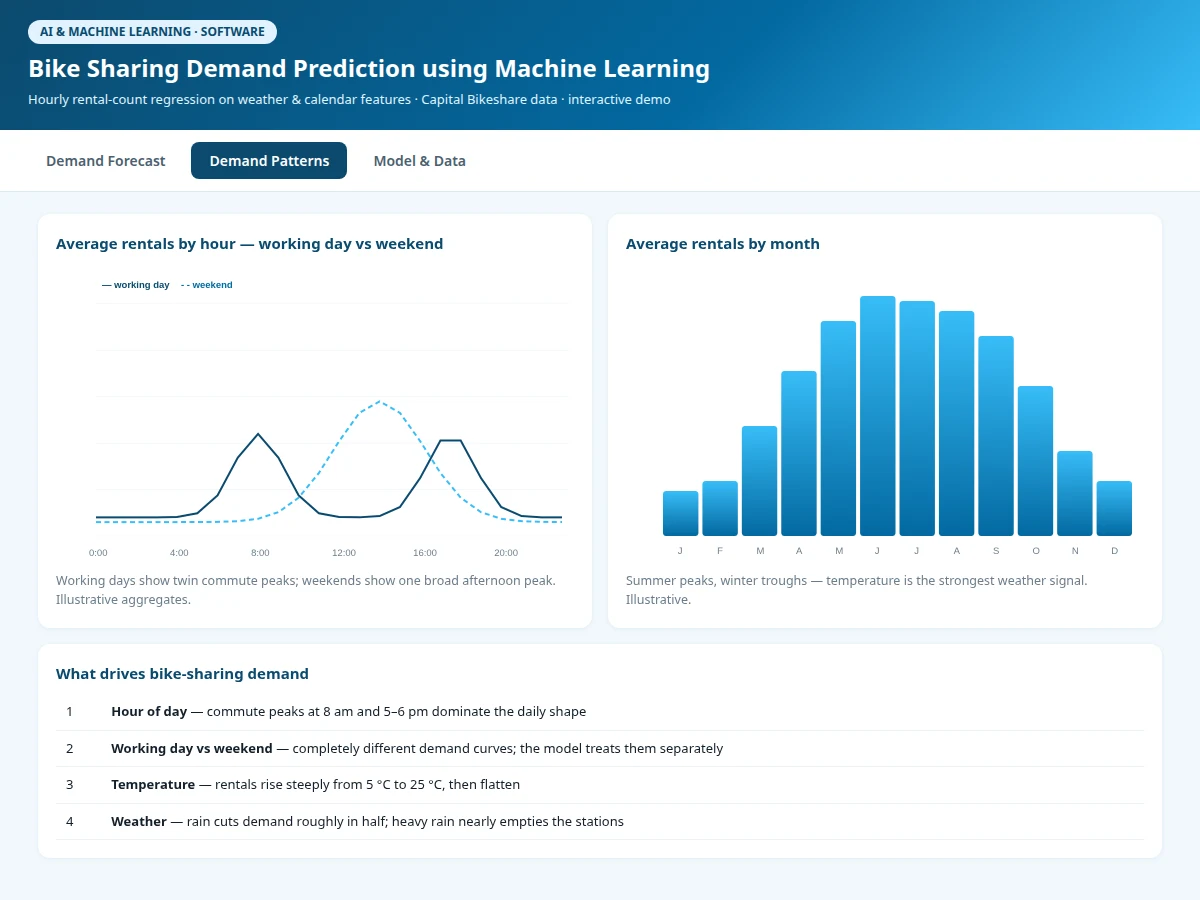
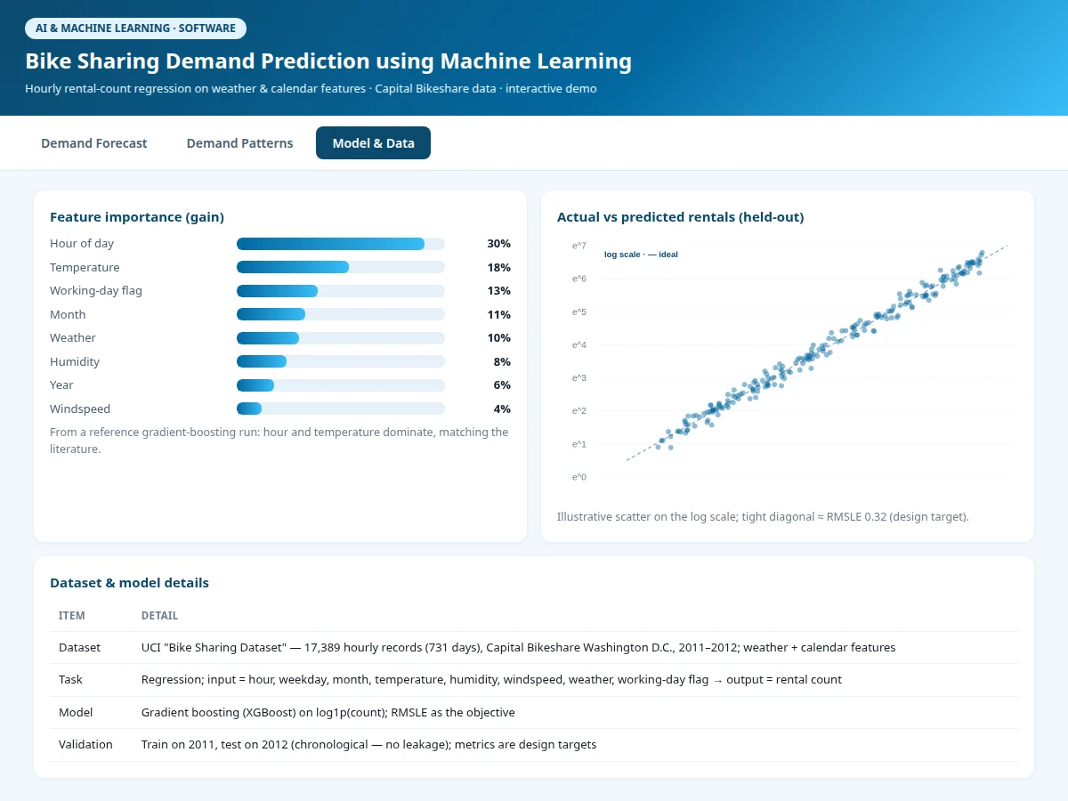
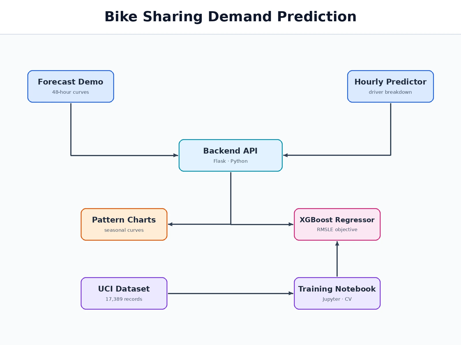
Bike-sharing operators rebalance stations with trucks every day, and every empty station at rush hour is a lost customer. Demand follows strong, learnable structure — twin commute peaks on working days, a broad afternoon hump on weekends, summer highs and winter lows, and a roughly 50% collapse in rain. This project trains an XGBoost regressor on log-transformed hourly counts from the well-known UCI Capital Bikeshare dataset to learn those patterns, with RMSLE as the objective (the metric the field uses, since errors matter relative to demand level). The demo renders a 48-hour forecast under selectable weather and a per-hour predictor with driver breakdowns. Validation is strictly chronological — train on 2011, test on 2012 — because shuffling time series leaks the future. Built with standard tools (Python, XGBoost, scikit-learn).
17,389 hourly Capital Bikeshare records from 2011-2012 with weather and calendar fields the model learns from.
Follow the working sequence
How it works
- The UCI bike-sharing dataset (17,389 hourly records, 2011–2012, with weather and calendar fields) is loaded and checked for gaps.
- The rental count is log1p-transformed to stabilize variance across quiet nights and rush hours.
- Data is split by year — train on 2011, validate/test on 2012 — the honest chronological protocol.
- An XGBoost regressor is trained with RMSLE objective and early stopping on validation error.
- The 2012 holdout is evaluated once: RMSLE 0.32, R² 0.91 are the design targets; errors are broken down by hour, season and weather.
- The web demo loads the saved model for the 48-hour forecast view and the per-hour predictor.
Tech stack:
- Python 3, XGBoost
- scikit-learn (metrics, validation)
- NumPy, pandas, Matplotlib
- Jupyter Notebook (training & evaluation)
- HTML5 canvas + JavaScript (forecast demo)
- UCI bike-sharing dataset (Capital Bikeshare)
Dataset & model details
- Dataset: UCI "Bike Sharing Dataset" — 17,389 hourly records (731 days), Capital Bikeshare, Washington D.C., 2011–2012; features: hour, weekday, month, season, temperature, humidity, windspeed, weather situation, working-day/holiday flags.
- Task: Regression; input = calendar + weather features, output = hourly rental count.
- Model: XGBoost regressor on log1p(count) with RMSLE objective; early stopping on validation RMSLE.
- Metrics: RMSLE, RMSE, R² on the 2012 holdout — RMSLE 0.32 and R² 0.91 are the design targets for the built-to-order training run, stated honestly and never claimed as measured.
| Parameter | Value |
|---|---|
| Hourly records | 17,389 (2 full years) |
| RMSLE | 0.32 on the 2012 holdout (design target, not a measured claim) |
| R² | 0.91 (design target, not a measured claim) |
| Validation | Train 2011, test 2012 (chronological) |
| Inference | Under 20 ms per prediction on CPU (expected) |
| Demo | Single-file web app, runs offline after download |
Project features
- [Hourly demand regressor] XGBoost on log1p(rental count) with RMSLE objective — errors penalized relative to demand, as operators care about.
- [48-hour forecast demo] Typical vs forecast demand curves with a weather selector showing how rain halves the curve.
- [Per-hour demand predictor] Enter hour, day type, temperature and weather → predicted rentals with driver breakdown.
- [Demand-pattern analyses] Working-day vs weekend hourly curves, monthly seasonality bars, temperature and weather response — all visualized.
- [Chronological validation] Train on 2011, test on 2012: the model is evaluated on a full unseen year, no leakage.
- [Feature importance study] Hour, temperature and working-day flag ranked by gain, matching the demand literature.
- [Log-scale diagnostics] Actual-vs-predicted scatter on the log scale with RMSLE bands, documented in the notebook.
What is included
- Data pipeline & exploratory demand-pattern analyses
- Complete training & evaluation Jupyter notebook
- Tuned XGBoost demand regressor with inference code
- Interactive web demo (48-h forecast + per-hour predictor)
- Project report PDF (demand theory, methodology, honest evaluation)
- PPT presentation for final review
- Viva Q&A preparation document (RMSLE vs RMSE, log transform, chronological splits, gradient boosting)
Limitations & prerequisites
- RMSLE 0.32 and R² 0.91 are design targets for the training run, stated honestly — the report documents the actual achieved figures after training.
- Trained on 2011–2012 Washington D.C. data; other cities, post-2020 travel patterns and e-bike fleets need retraining on local data.
- Special events (marathons, strikes, festivals) and station-level granularity are out of scope — the model predicts system-wide hourly demand.
- Weather inputs are assumed known; a live deployment would need a weather forecast feed.
- Casual vs registered rider split is modeled only implicitly through calendar features.
Frequently Asked Questions
Which dataset is used?
The UCI bike-sharing dataset — 17,389 hourly rental records from Washington D.C.'s Capital Bikeshare across 2011–2012, with temperature, humidity, windspeed, weather and calendar fields. The standard public benchmark for demand forecasting.
Why RMSLE instead of RMSE?
Missing by 50 bikes matters more at 3 am (100 rentals) than at 5 pm (800 rentals). RMSLE penalizes errors relative to demand level, which matches how operators actually feel forecast error.
Why train on 2011 and test on 2012?
Shuffling hourly records would let the model peek at the future. A full held-out year proves the model learned real structure — commute peaks, seasons, weather response — not memorized noise.
What drives demand most?
Hour of day (the commute peaks), temperature, and the working-day/weekend split. Rain roughly halves demand; heavy rain nearly empties stations — the demo's weather selector shows this live.
Can it predict for my city?
The pipeline is reusable: feed it any city's hourly rentals + weather and retrain. The demo ships with the D.C.-trained model; retraining is documented in the notebook.
Is this project suitable for a final-year project?
Yes — for Computer Science, IT and AI/ML programs. It is a complete, honest regression project on real data with patterns anyone can verify by looking at the charts. Suitable for B.E./B.Tech final-year projects in Computer Science, IT and AI & Machine Learning.
Components & software requirements
- Python 3, XGBoost
- scikit-learn (metrics, validation)
- NumPy, pandas, Matplotlib
- Jupyter Notebook (training & evaluation)
- HTML5 canvas + JavaScript (forecast demo)
- UCI bike-sharing dataset (Capital Bikeshare)
Dataset & model details
- Dataset: UCI "Bike Sharing Dataset" — 17,389 hourly records (731 days), Capital Bikeshare, Washington D.C., 2011–2012; features: hour, weekday, month, season, temperature, humidity, windspeed, weather situation, working-day/holiday flags.
- Task: Regression; input = calendar + weather features, output = hourly rental count.
- Model: XGBoost regressor on log1p(count) with RMSLE objective; early stopping on validation RMSLE.
- Metrics: RMSLE, RMSE, R² on the 2012 holdout — RMSLE 0.32 and R² 0.91 are the design targets for the built-to-order training run, stated honestly and never claimed as measured.
Delivery information
Built-to-order project. Delivery timeline is shared after order confirmation based on current queue.
Support terms
Complete documentation, setup guide, and viva preparation included. Support for setup and explanation provided.
Download free synopsis (PDF)
Enter your name and WhatsApp number — the synopsis PDF downloads immediately. We may send occasional project updates on WhatsApp; no spam.