
More project photos (2)
The problem
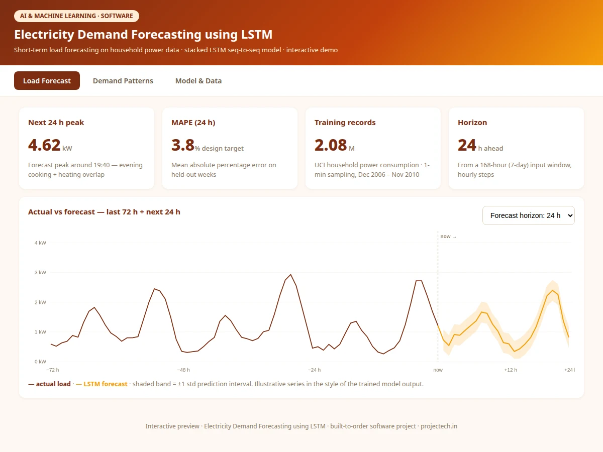
Grid operators and utilities live or die by short-term load forecasts — overestimate and generators idle expensively, underestimate and the grid strains. Yet most student forecasting projects shuffle time series randomly into train/test splits, leaking the future into training and reporting fantasy accuracy. This project does it honestly: a stacked LSTM reads a 168-hour window of minute-aggregated household demand plus calendar features and emits the next 24 hourly values in one seq-to-seq pass, trained and tested on strictly chronological splits of the well-known UCI household power consumption dataset. The demo plots actual vs forecast load with prediction intervals and lets you change the horizon. Everything — the double daily peak, the weekend shape, the LSTM gate mechanics — is explainable with standard tools (Python, TensorFlow/Keras).
How it works
- The UCI household power data (2,075,259 minute-level records, Dec 2006 – Nov 2010) is resampled to hourly demand and cleaned of gaps.
- Calendar features (hour, weekday, month) and lag features are engineered; sequences of 168 hours become model inputs with the next 24 hours as targets.
- Data is split chronologically — train up to end-2009, validate/test on 2010 — so the model is always tested on a future it never saw.
- The stacked LSTM (64 → dropout 0.2 → 32 → dense 24) is trained with Adam on MSE loss, early-stopping on validation MAPE.
- Held-out weeks are evaluated with MAPE, RMSE and MAE per horizon; errors are analyzed by hour of day and season.
- The web demo loads the trained weights, takes the latest window, and renders actual vs forecast with prediction intervals.
Tech stack:
- Python 3, TensorFlow/Keras
- NumPy, pandas, Matplotlib
- scikit-learn (scaling, metrics)
- Jupyter Notebook (training & evaluation)
- HTML5 canvas + JavaScript (forecast demo)
- UCI household power dataset
Dataset & model details
- Dataset: UCI "Individual household electric power consumption" — 2,075,259 one-minute measurements (global active/reactive power, 3 sub-meterings), Dec 2006 – Nov 2010, one household in Sceaux, France.
- Task: Multivariate sequence regression; input = 168-hour window × 6 features, output = next 24 hourly kW values.
- Model: Stacked LSTM: LSTM(64, return_sequences) → Dropout(0.2) → LSTM(32) → Dense(24, linear); approximately 45k parameters; Adam optimizer, MSE loss.
- Metrics: MAPE, RMSE, MAE per horizon on the chronological holdout — 3.8% MAPE at 24 h is the design target for the built-to-order training run, stated honestly and never claimed as measured.
| Parameter | Value |
|---|---|
| Input window | 168 hours × 6 features |
| Forecast horizon | 24 hours (48 h demo mode) |
| Model parameters | Approximately 45,000 (design target) |
| MAPE at 24 h | 3.8% (design target, not a measured claim) |
| Training time | Approximately 20–40 min on a laptop CPU (expected) |
| Inference | Under 50 ms per forecast on CPU (expected) |
| Demo | Single-file web app, runs offline after download |
Project features
- [Stacked LSTM forecaster] Two LSTM layers (64 → 32 units) with dropout, emitting 24 hourly steps at once so the forecast keeps a coherent daily shape.
- [168-hour input window] A full week of context lets the model learn both daily peaks and weekday/weekend differences.
- [Chronological validation] Train on 2006–2009, test on 2010 — no shuffling, no leakage, the honest protocol for time series.
- [Prediction intervals] The demo shades ±1 std bands around the forecast so uncertainty is visible, not hidden.
- [Interactive horizon control] Switch between 24 h and 48 h forecasts and watch error grow with horizon, as theory predicts.
- [Training-curve diagnostics] Loss plots with early stopping documented in the notebook and report.
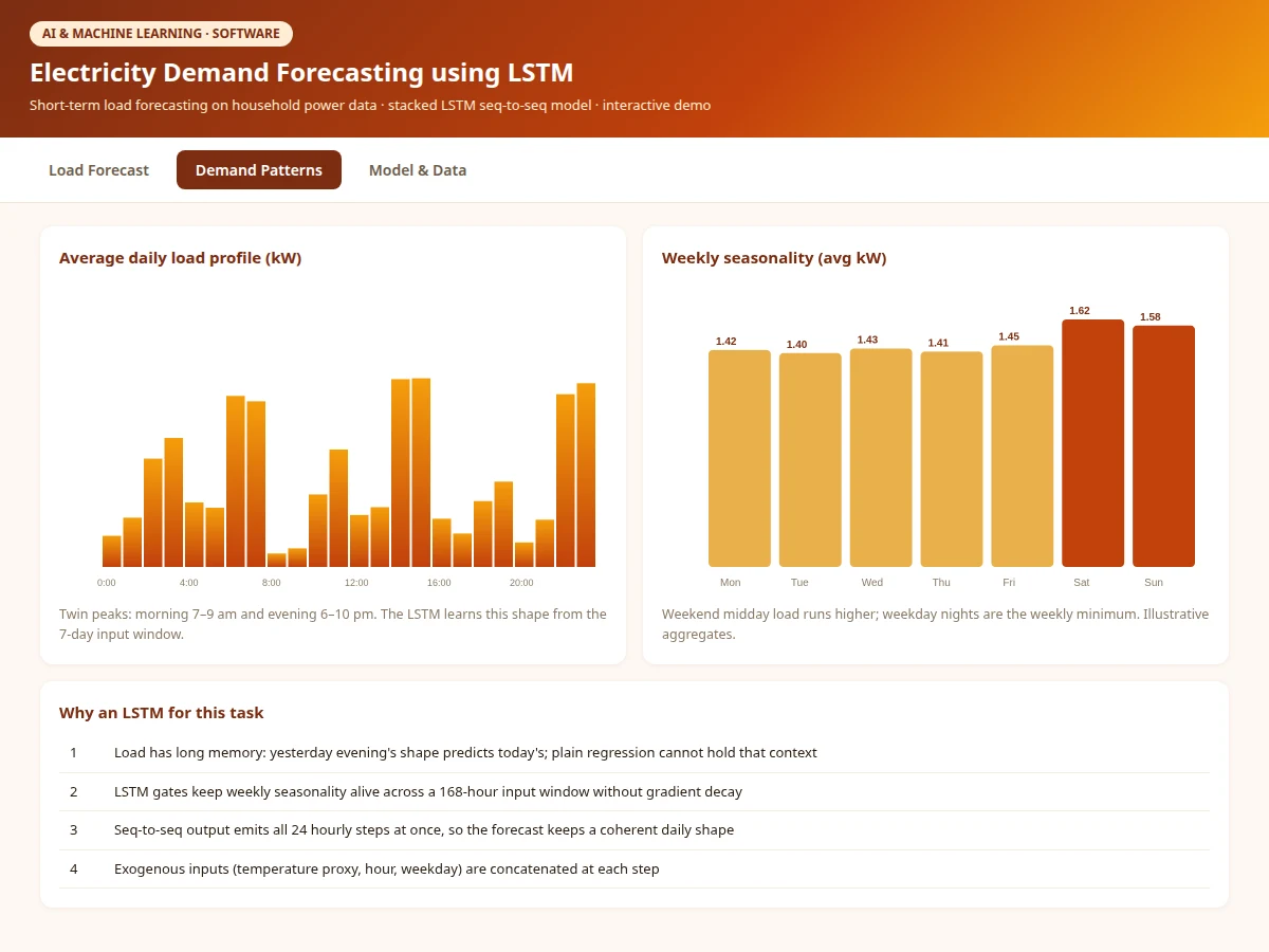
- [Feature analysis] Calendar and lag features ranked; the double-peak daily profile and weekly seasonality visualized.
What is included
- Data cleaning & feature-engineering pipeline
- Complete training & evaluation Jupyter notebook
- Trained stacked-LSTM model weights with inference code
- Interactive forecast web demo (actual vs forecast + intervals)
- Project report PDF (time-series theory, LSTM design, honest evaluation)
- PPT presentation for final review
- Viva Q&A preparation document (LSTM gates, seq-to-seq, leakage, MAPE vs RMSE)
Limitations & prerequisites
- Trained on a single French household — the learned daily shape will not transfer directly to Indian households or industrial feeders without retraining.
- 3.8% MAPE is a design target for the training run, stated honestly — the report documents the actual achieved figure after training.
- Extreme events (heatwaves, blackouts, holidays) are rare in training data and forecast less reliably; the intervals communicate this.
- The model uses only consumption history and calendar features — no weather inputs, which would help and are listed as future scope.
- Minute-level data is aggregated to hourly; sub-hourly spikes are out of scope.
Frequently Asked Questions
Which dataset is used and why?
The UCI household power consumption dataset — over 2 million minute-level records across four years. It is the standard public benchmark for residential load forecasting, long enough to learn weekly and seasonal structure.
Why an LSTM instead of simple regression?
Load has long memory: this evening's shape depends on the whole past week. LSTM gates carry that context across the 168-hour window; plain regression and ARIMA-style models either forget it or need heavy manual feature work.
How do you avoid leaking the future into training?
Strictly chronological splits — the model trains on 2006–2009 and is tested on 2010. Random shuffling, the common student mistake, is explicitly avoided and the report explains why.
What do the shaded bands on the forecast mean?
±1 standard-deviation prediction intervals from the validation residuals. They show where the model is confident (night valleys) and where it isn't (evening peaks).
Can it forecast for my own home?
The pipeline is reusable: point it at any hourly meter series and retrain. The demo ships with the UCI-trained model; retraining on new data is documented in the notebook.
Is this project suitable for a final-year project?
Yes — for Electrical, Computer Science, IT and AI/ML programs. It demonstrates sequence modeling, honest time-series evaluation, and a working forecast product. Suitable for B.E./B.Tech final-year projects in Electrical, Computer Science, IT and AI & Machine Learning.
Components & software requirements
- Python 3, TensorFlow/Keras
- NumPy, pandas, Matplotlib
- scikit-learn (scaling, metrics)
- Jupyter Notebook (training & evaluation)
- HTML5 canvas + JavaScript (forecast demo)
- UCI household power dataset
Dataset & model details
- Dataset: UCI "Individual household electric power consumption" — 2,075,259 one-minute measurements (global active/reactive power, 3 sub-meterings), Dec 2006 – Nov 2010, one household in Sceaux, France.
- Task: Multivariate sequence regression; input = 168-hour window × 6 features, output = next 24 hourly kW values.
- Model: Stacked LSTM: LSTM(64, return_sequences) → Dropout(0.2) → LSTM(32) → Dense(24, linear); approximately 45k parameters; Adam optimizer, MSE loss.
- Metrics: MAPE, RMSE, MAE per horizon on the chronological holdout — 3.8% MAPE at 24 h is the design target for the built-to-order training run, stated honestly and never claimed as measured.
Delivery information
Built-to-order project. Delivery timeline is shared after order confirmation based on current queue.
Support terms
Complete documentation, setup guide, and viva preparation included. Support for setup and explanation provided.