
More project photos (2)
The problem
Loan default prediction with Random Forest and SHAP explanations tackles a lending problem: a lender must judge, before money is disbursed, whether a borrower will repay or stop paying. Traditional scorecards use a handful of hand-set rules, so they miss interactions — for example, a moderate income looks safe until it is combined with a high interest rate and a high debt-to-income ratio. A Random Forest learns those interactions from thousands of past loans instead, because each tree splits on different features and the forest votes on the outcome. The catch is opacity: a vote share alone does not tell a reviewer why one applicant was flagged and another was not. SHAP explanations close that gap by sharing the prediction fairly among the applicant's features, so every decision can be inspected, challenged and documented. That combination makes the system useful as a teaching build and a demonstration of responsible credit modelling.
Lenders, banks and peer-to-peer platforms all face the same asymmetry: approving a loan that defaults loses principal, while rejecting a loan that would have repaid loses interest income. A model that only outputs a score hides which side of that trade-off drove the decision, and a reviewer cannot defend or overturn it. This build therefore treats explanation as a first-class output, not an add-on chart: every prediction ships with its ranked feature contributions, a probability, and a Low, Review or High band. The result is a system a student can walk through end to end — from raw loan records to a justified decision — and a reviewer can interrogate feature by feature.
This is a built-to-order software project: the training notebook, trained model, explanation outputs, web demo and the complete documentation set are prepared fresh for you.
Concept
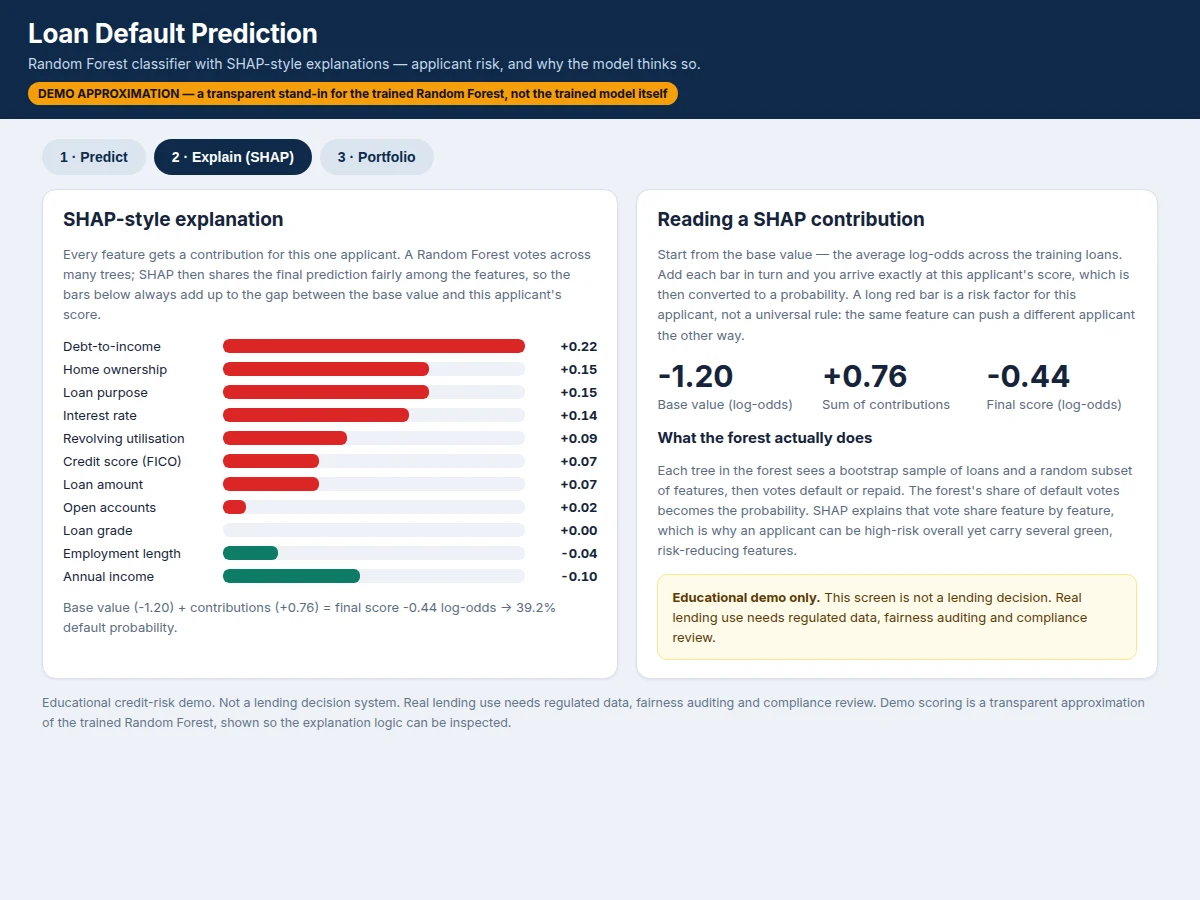
The concept has two halves that must be understood together. A Random Forest is an ensemble of decision trees: each tree is trained on a different bootstrap sample of loans and a random subset of features, and the forest's prediction is the share of trees voting for default. SHAP (SHapley Additive exPlanations) then explains that vote share by distributing it fairly among the features, using the game-theoretic Shapley value: each feature's contribution is its average marginal effect across all possible feature orderings. Because the contributions are additive, they sum exactly to the gap between the average prediction and the applicant's own prediction — which is why a SHAP bar chart can be read as a complete account of one decision, not a rough ranking.
An applicant profile with loan and credit details.
Follow the working sequence
How it works
Loan default prediction with Random Forest and SHAP explanations works end to end in four stages. First, applicant and loan features — amount, income, interest rate, debt-to-income ratio, credit score, employment length, revolving utilisation, open accounts, grade, home ownership and purpose — are cleaned, encoded and scaled into the eleven inputs the model expects. Second, a Random Forest is trained on historical LendingClub loans, where hundreds of decision trees each learn from a different sample of loans and features, then vote on whether a new loan will be repaid or charged off. Third, the share of trees voting for default becomes the predicted probability, mapped to a Low, Review or High band for presentation. Fourth, SHAP values decompose that probability feature by feature, producing a ranked list of contributions that sum exactly to the gap between the average prediction and the applicant's own score.
- Closed LendingClub loans are loaded and filtered to the two completed outcomes, Fully Paid and Charged Off, discarding loans still in progress whose outcome is unknown.
- The eleven modelling features are selected, missing values are handled, categorical fields (grade, home ownership, purpose) are encoded, and leakage fields such as post-outcome payment totals are excluded.
- The data is split with stratification so the train and test sets carry the same default rate, and class weights are set to balanced so minority defaults are not ignored.
- A Random Forest of 300 trees (design target) is trained with cross-validation used to check the depth, leaf-size and feature-subset settings before the final fit.
- The held-out test set is evaluated once with a confusion matrix, ROC-AUC, PR-AUC and per-class precision, recall and F1, and the decision threshold and risk bands are fixed from those results.
- SHAP TreeExplainer values are computed for test predictions and for any new applicant, producing the ranked contribution chart shown in the demo.
- In the web demo, an applicant profile is scored through the same eleven-feature pipeline and displayed with its probability, risk band and SHAP contributions.
Tech stack:
- Python 3, scikit-learn (Random Forest)
- SHAP TreeExplainer
- pandas, NumPy (data preparation)
- LendingClub loan data via Kaggle
- Jupyter Notebook (training & evaluation)
- HTML, CSS, JavaScript (scoring & explanation demo)
- Matplotlib, Seaborn (evaluation plots)
Dataset & model details
- Dataset: LendingClub Loan Data, via Kaggle — a large public file of historical peer-to-peer loans; published Kaggle versions range from roughly 890,000 to 2.2 million rows with 150 or more columns depending on the version, so the build documents the exact version used at training time. The build uses the closed-loan subset only, i.e. loans whose outcome is known. Classes: 2 — Fully Paid (loan repaid, label 0) and Charged Off (loan defaulted and written off, label 1).
- Task: Binary classification; input = 11 applicant and loan features (amount, income, interest rate, debt-to-income ratio, credit score, employment length, revolving utilisation, open accounts, grade, home ownership, purpose); output = default probability from 0% to 100% plus a Low / Review / High band.
- Model: Random Forest classifier, 300 trees (design target), trained on the closed-loan subset with balanced class weights; the demo's scoring rule is a transparent approximation of the trained forest, labelled as such inside the demo, while the delivered notebook trains and explains the real forest with SHAP TreeExplainer.
- Metrics: ROC-AUC, PR-AUC, confusion matrix, per-class precision, recall and F1. No accuracy is claimed as measured: the built-to-order training run reports the achieved figures, against a design target of ROC-AUC above 0.75.
| Parameter | Value |
|---|---|
| Input features | 11 features (count) |
| Classes | 2 classes: Fully Paid and Charged Off |
| Model | Random Forest with 300 trees (design target) |
| Training data | LendingClub file via Kaggle (row count varies by version, roughly 890,000 to 2.2 million rows); closed-loan subset used for training |
| Output | Default probability from 0% to 100% plus Low / Review / High band |
| Risk bands | Below 30% Low, 30–60% Review, above 60% High (configurable thresholds) |
| Demo response | Expected: under 1 second per prediction (browser demo, JavaScript scoring) |
| Explanation method | SHAP TreeExplainer on the trained forest (delivered build); SHAP-style additive contributions in the browser demo (labelled approximation) |
| Evaluation | ROC-AUC, PR-AUC, confusion matrix, per-class precision/recall/F1 (reported after the training run) |
| Demo format | Single-file web app, runs offline after download |
Project features
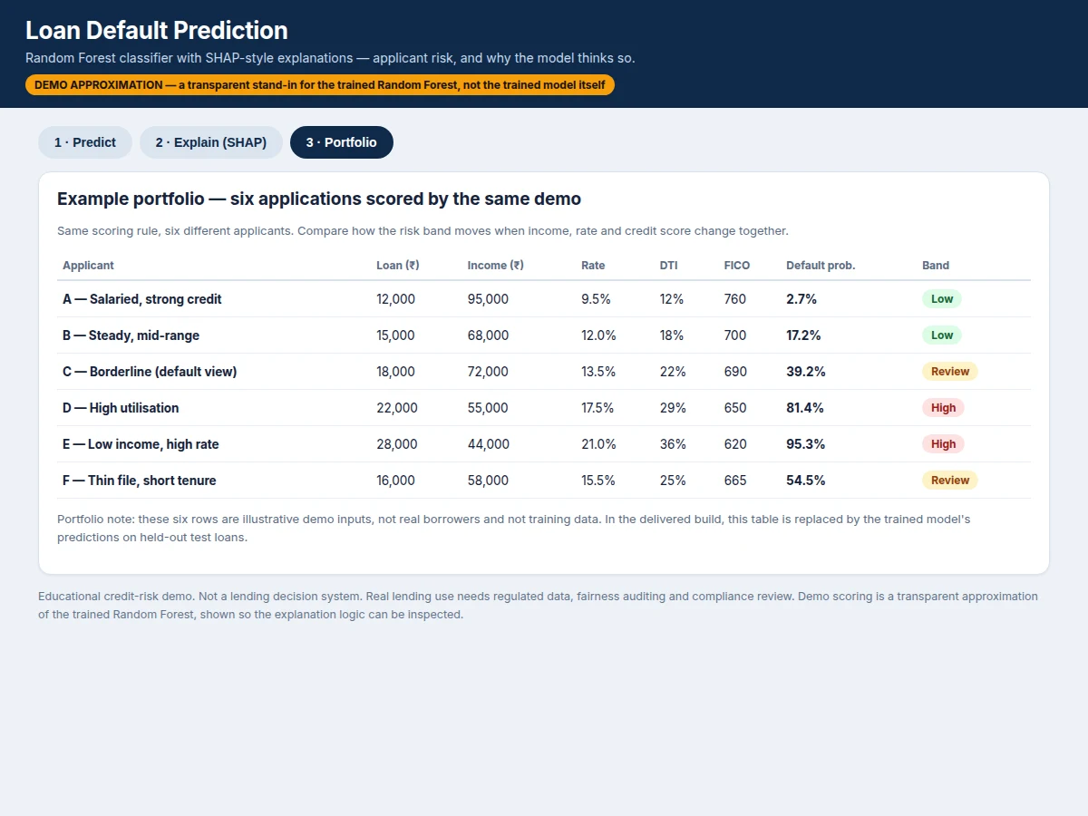
Loan default prediction with Random Forest and SHAP explanations ships as a complete, inspectable credit-risk build: a trained Random Forest, a SHAP explanation for every prediction, and a web demo that scores any applicant profile on demand. The classifier takes eleven applicant and loan features — amount, income, interest rate, debt-to-income ratio, credit score, employment length, revolving utilisation, open accounts, grade, home ownership and purpose — and returns a default probability with a Low, Review or High band. The explanation panel then ranks each feature by its contribution, so a reviewer sees exactly what pushed the score up or down instead of trusting a bare number. A portfolio view scores six illustrative applicants side by side, showing how risk moves when income, rate and credit score change together. Together, these capabilities let a student demonstrate training, evaluation, explanation and presentation in one coherent build.
- [Random Forest classifier] An ensemble of decision trees trained on historical loan records, returning a default probability rather than a bare yes/no label, so borderline applicants stay visible instead of being forced into a hard class.
- [SHAP explanation for every prediction] Each prediction is decomposed into per-feature contributions that sum to the gap between the average prediction and the applicant's score, rendered as a ranked bar chart with a plain-language reading guide.
- [Interactive applicant scoring demo] A single-file web demo with eleven applicant inputs, three preset profiles (low-risk, borderline, high-risk) and instant scoring, so any profile can be tested and explained without running code.
- [Class-imbalance handling] Defaults are the minority class, so the build uses a stratified train/test split, balanced class weights and class-aware evaluation instead of headline accuracy alone, which would flatter a model that simply predicts "repaid" for everyone.
- [Threshold and risk banding] The default probability is mapped to Low (below 30%), Review (30–60%) and High (above 60%) bands, with the decision threshold documented and adjustable, so the trade-off between missed defaults and false alarms is explicit.
- [Portfolio comparison view] Six illustrative applicants are scored side by side in the demo, showing how the band moves when income, interest rate and credit score change together.
- [Evaluation report] Confusion matrix, ROC-AUC, PR-AUC and per-class precision, recall and F1, plus forest feature importance and a SHAP summary plot, all documented for the review discussion.
Optional customisation (not in the base build): a custom institutional dataset swap, a calibration curve and probability calibration, a fairness slice report across applicant groups, and a Flask API deployment of the trained model. Future scope (not implemented): online learning on new loans, bureau-data integration, and a mobile applicant-entry app.
Builder note, measured from the demo build: the preset borderline applicant (loan 18,000, income 72,000, interest rate 13.5%, debt-to-income 22%, credit score 690) scored 39.2% default probability in the working demo, in the Review band, with debt-to-income as its largest single push toward default at +0.22 log-odds; the demo's own arithmetic reads base value -1.20 plus contributions +0.76 equals a final score of -0.44 log-odds.
What is included
- Complete training & evaluation Jupyter notebook (data loading, filtering, preprocessing, training, evaluation, SHAP analysis)
- Trained Random Forest model file with the preprocessing pipeline
- Interactive web demo: applicant scoring, SHAP explanation view and portfolio comparison view
- Evaluation report: confusion matrix, ROC-AUC, PR-AUC, per-class metrics, feature importance and SHAP summary plot
- Project report PDF (background, Random Forest theory, SHAP method, methodology, results, limitations)
- PPT presentation for final review
- Review Q&A preparation document (ensembles, bagging, Shapley values, class imbalance, threshold trade-offs)
Requirements
- Python 3 with scikit-learn, SHAP, pandas, NumPy, Matplotlib and Seaborn (listed in a requirements file)
- Jupyter Notebook for the training run; any modern browser for the demo (no server needed)
- Approximately 2 GB of free disk space for the dataset and model artefacts (expected)
- A laptop with approximately 8 GB of RAM for the full training run (expected); the demo runs on any machine that opens the HTML file
Limitations & prerequisites
- This is an educational credit-risk demonstration, not a lending decision system: real lending use needs regulated data, fairness auditing and compliance review before any applicant is judged.
- The LendingClub file used is a historical snapshot, so its patterns may not reflect current lending conditions or other lenders' portfolios.
- Historical lending data can encode past approval biases; the build reports overall metrics but does not by itself prove fairness across applicant groups — a fairness slice report is an optional extra.
- The browser demo's scoring rule is a transparent approximation of the trained forest, labelled inside the demo; demo probabilities are illustrative, and only the notebook's trained model figures count as the build's results.
- SHAP explains the model's reasoning, not the real-world cause of a default: a large contribution means the feature moved the prediction, not that changing it would change the borrower's behaviour.
- Performance varies with the file version, the train/test split and the forest settings; the design target of ROC-AUC above 0.75 is a target, not a measured claim.
- The model uses only the eleven listed features; it has no access to bank statements, employment verification or bureau history beyond what the dataset contains.
Timeline
- Indicative build timeline, approximately 3 weeks in total: Week 1 — dataset acquisition, filtering and baseline model; Week 2 — forest tuning, evaluation and threshold/band setting; Week 3 — SHAP analysis, web demo, report and presentation. Timelines shift with dataset download access and review feedback.
Support
- Setup help for the notebook environment and the demo, a walkthrough of the SHAP reading guide, and corrections support for report or presentation issues found during the review cycle. Support covers the delivered build; new features beyond the listed scope are handled as customisation.
Frequently Asked Questions
Which dataset is used and why?
The build uses LendingClub loan data from Kaggle, filtered to closed loans whose outcome is known: Fully Paid or Charged Off. It is the standard public dataset for this task, with hundreds of thousands of real historical loans and the applicant, loan and credit features a default model genuinely needs. The full file is large, so the build documents exactly which subset and which eleven features were used, and excludes post-outcome fields that would leak the answer.
Why a Random Forest instead of a single decision tree or logistic regression?
A single tree overfits and a linear model misses feature interactions, while a forest averages hundreds of trees trained on different loan samples and feature subsets. That averaging stabilises predictions on tabular credit data and gives a natural probability from the share of trees voting for default. The trade-off is opacity, which is exactly why SHAP explanations are part of the build rather than an optional chart.
How does SHAP explain a single prediction?
SHAP shares the prediction fairly among the applicant's features using Shapley values, so each feature receives a contribution in log-odds that pushes the score toward or away from default. The contributions are additive: base value plus all contributions equals the applicant's final score, which converts to the displayed probability. A long red bar is therefore a complete, checkable reason for that one decision, not a global claim about all borrowers.
Is the accuracy guaranteed?
No accuracy figure is guaranteed or claimed as measured before the training run is executed for the order. The build reports the achieved ROC-AUC, PR-AUC, confusion matrix and per-class metrics on the held-out test set, against a stated design target of ROC-AUC above 0.75. If the achieved figures fall short of the target, the report says so and the tuning section records what was tried.
Can this model approve or reject real loans?
No — as delivered, this build cannot approve or reject real loans. It is an educational demonstration trained on historical public data, and real lending decisions need regulated data, fairness auditing, adverse-action reasoning and compliance review that this build does not provide. Any production use would also need current, consented data and a full governance process; the demo and report both carry this limit plainly.
Is this project suitable for a final-year project?
Yes — it fits Computer Science, AI & Machine Learning and IT programmes, and demonstrates ensemble learning, class-imbalance handling, evaluation discipline and model explainability in one build. The SHAP analysis gives the review discussion a concrete, visual anchor: the student can defend not just what the model predicted, but why it predicted it for a specific applicant.
Components & software requirements
- Python 3, scikit-learn (Random Forest)
- SHAP TreeExplainer
- pandas, NumPy (data preparation)
- LendingClub loan data via Kaggle
- Jupyter Notebook (training & evaluation)
- HTML, CSS, JavaScript (scoring & explanation demo)
- Matplotlib, Seaborn (evaluation plots)
Dataset & model details
- Dataset: LendingClub Loan Data, via Kaggle — a large public file of historical peer-to-peer loans; published Kaggle versions range from roughly 890,000 to 2.2 million rows with 150 or more columns depending on the version, so the build documents the exact version used at training time. The build uses the closed-loan subset only, i.e. loans whose outcome is known. Classes: 2 — Fully Paid (loan repaid, label 0) and Charged Off (loan defaulted and written off, label 1).
- Task: Binary classification; input = 11 applicant and loan features (amount, income, interest rate, debt-to-income ratio, credit score, employment length, revolving utilisation, open accounts, grade, home ownership, purpose); output = default probability from 0% to 100% plus a Low / Review / High band.
- Model: Random Forest classifier, 300 trees (design target), trained on the closed-loan subset with balanced class weights; the demo's scoring rule is a transparent approximation of the trained forest, labelled as such inside the demo, while the delivered notebook trains and explains the real forest with SHAP TreeExplainer.
- Metrics: ROC-AUC, PR-AUC, confusion matrix, per-class precision, recall and F1. No accuracy is claimed as measured: the built-to-order training run reports the achieved figures, against a design target of ROC-AUC above 0.75.
Delivery information
Built-to-order project. Delivery timeline is shared after order confirmation based on current queue.
Support terms
Complete documentation, setup guide, and viva preparation included. Support for setup and explanation provided.
Download free synopsis (PDF)
Enter your name and WhatsApp number — the synopsis PDF downloads immediately. We may send occasional project updates on WhatsApp; no spam.