
More project photos (2)

The problem
Testing budgets are finite and codebases are not: in any large project, a small fraction of modules hides most of the bugs. If you could predict which modules those are from static measurements alone — lines of code, decision density, operator complexity — you could point reviewers and testers exactly where they matter. That is software defect prediction, and this project implements it on the classic NASA Metrics Data Program datasets (CM1, KC1, JM1 and others) from the PROMISE repository: thousands of real software modules, each described by McCabe and Halstead metrics and labeled defective or clean. A random-forest classifier learns which metric patterns precede defects, evaluated with AUC and cross-project validation — training on one project and testing on another, the honest test of whether the patterns generalize.
How it works
- NASA MDP datasets (CM1: 498 modules, KC1: 2,109, JM1: 10,885) are loaded with their static metrics and defect labels.
- Metric distributions are explored; skewed Halstead metrics are log-transformed with the choice documented.
- A random-forest classifier trains on the metric vectors, with stratified cross-validation and class weighting for the defective minority.
- Within-project evaluation reports AUC, precision/recall and the confusion matrix; cross-project runs test generalization across datasets.
- Permutation importance ranks the metrics, revealing which complexity measures actually signal defects.
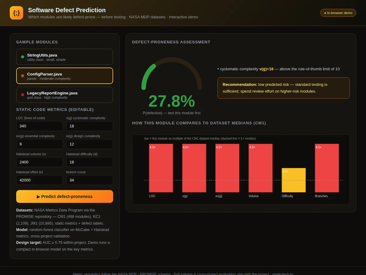
- In the demo, entered metrics are fed through the saved model; the app shows P(defective), the driver metrics and a prioritized testing recommendation.
Tech stack:
- Python 3, scikit-learn (random forest)
- Pandas, NumPy (data handling)
- Matplotlib (distributions, ROC curves)
- Jupyter Notebook (training & evaluation)
- HTML5 canvas + JavaScript (interactive demo)
- NASA MDP datasets (PROMISE repository)
Dataset & model details
- Dataset: NASA Metrics Data Program datasets via the PROMISE repository — CM1 (498 modules), KC1 (2,109 modules), KC2, PC1 and JM1 (10,885 modules); each module described by McCabe (LOC, v(g), ev(g), iv(g)) and Halstead (n, v, l, d, i, e, b, t) metrics with a binary defective/clean label.
- Task: Binary classification; input = static code-metric vector per module, output = P(defective).
- Model: Random forest (200 trees, class-weighted), with log-transformed skewed metrics; hyperparameters selected by stratified cross-validation.
- Metrics: AUC ≥ 0.75 within-project (design target for the built-to-order training run), plus precision/recall at the operating threshold and cross-project AUC. Published defect-prediction studies report AUC around 0.70–0.80 on these datasets; no figure is claimed as measured until the training run is executed for the order.
| Parameter | Value |
|---|---|
| Input | ~20 static code metrics per module |
| Output | P(defective), binary risk flag |
| Labeled modules | 498–10,885 per dataset (CM1–JM1) |
| AUC | ≥ 0.75 within-project (design target, not a measured claim) |
| Training time | Approximately 2–10 min on a laptop CPU (expected) |
| Inference | Sub-millisecond per module on CPU (expected) |
| Model file | Approximately 5–20 MB (expected) |
| Demo | Single-file web app, runs offline after download |
Project features
- [Defect-proneness classifier] Random forest over McCabe (cyclomatic, essential, design complexity) and Halstead (volume, difficulty, effort) metrics, outputting P(defective) per module.
- [Interactive module inspector] Enter any module's metrics — or load the sample "god class" — and get a risk score with the exact metrics driving it.
- [Dataset-median comparison chart] Each module's metrics plotted against dataset medians, making "this module is 4× more complex than typical" visible at a glance.
- [Cross-project validation] The model is tested training on one NASA dataset and predicting on another, documenting honestly how well defect patterns transfer.
- [Full training notebook] Data loading, metric distributions, imbalance handling, model training, within- and cross-project evaluation in one reproducible notebook.
- [Metric-importance analysis] Which metrics actually predict defects (and which are noise) ranked and explained for the report.
- [Exported trained model] Saved model plus the metric-computation guide, so new modules can be scored without retraining.
What is included
- Complete training & evaluation Jupyter notebook
- Trained random-forest model with metric preprocessing code
- Interactive module-risk web demo
- ROC curves, metric-importance plots, cross-project tables
- Project report PDF (background, metrics theory, methodology, results, generalization limits)
- PPT presentation for final review
- Viva Q&A preparation document (McCabe vs Halstead, AUC vs accuracy, class imbalance, cross-project validity)
Limitations & prerequisites
- Static metrics miss defects that come from requirements or integration issues — the report states what the model can and cannot see.
- Cross-project prediction is weaker than within-project; the honest numbers are reported, not hidden.
- AUC ≥ 0.75 is a design target for the training run, stated honestly — the report documents the actual achieved figure after training.
- The demo's in-browser model is a compact illustration on key metrics; the full random forest ships separately.
- A risk score prioritizes testing; it does not prove a module bug-free — no such claim is made.
Frequently Asked Questions
Which datasets are used and why?
The NASA MDP datasets (CM1, KC1, JM1…) from the PROMISE repository — the most-used public defect-prediction benchmarks, with real modules, standard metric sets and defect labels from actual QA histories.
What are McCabe and Halstead metrics?
McCabe metrics measure control-flow complexity (cyclomatic complexity counts independent paths); Halstead metrics measure code volume and mental effort from operator/operand counts. Both are computable without running the code.
Why AUC instead of accuracy?
Defective modules are a minority, so a lazy "all clean" model scores high accuracy while finding nothing. AUC measures ranking quality across all thresholds — the right metric for prioritization.
What is cross-project validation?
Training on one project's modules and testing on a different project's — the realistic deployment scenario, and much harder than testing on held-out modules of the same project. The report shows both.
How does the demo decide its recommendation?
It combines the predicted probability with the driver metrics: a 90%-risk module with v(g)=67 gets "test first"; a 15%-risk module gets "standard testing suffices."
Is this project suitable for a final-year project?
Yes — for AI & Machine Learning, Computer Science and IT programs. It connects software engineering with machine learning, uses real NASA data, and teaches honest evaluation including cross-project generalization. Suitable for B.E./B.Tech final-year projects in AI & Machine Learning, Computer Science and IT.
Components & software requirements
- Python 3, scikit-learn (random forest)
- Pandas, NumPy (data handling)
- Matplotlib (distributions, ROC curves)
- Jupyter Notebook (training & evaluation)
- HTML5 canvas + JavaScript (interactive demo)
- NASA MDP datasets (PROMISE repository)
Dataset & model details
- Dataset: NASA Metrics Data Program datasets via the PROMISE repository — CM1 (498 modules), KC1 (2,109 modules), KC2, PC1 and JM1 (10,885 modules); each module described by McCabe (LOC, v(g), ev(g), iv(g)) and Halstead (n, v, l, d, i, e, b, t) metrics with a binary defective/clean label.
- Task: Binary classification; input = static code-metric vector per module, output = P(defective).
- Model: Random forest (200 trees, class-weighted), with log-transformed skewed metrics; hyperparameters selected by stratified cross-validation.
- Metrics: AUC ≥ 0.75 within-project (design target for the built-to-order training run), plus precision/recall at the operating threshold and cross-project AUC. Published defect-prediction studies report AUC around 0.70–0.80 on these datasets; no figure is claimed as measured until the training run is executed for the order.
Delivery information
Built-to-order project. Delivery timeline is shared after order confirmation based on current queue.
Support terms
Complete documentation, setup guide, and viva preparation included. Support for setup and explanation provided.