
More project photos (2)
The problem
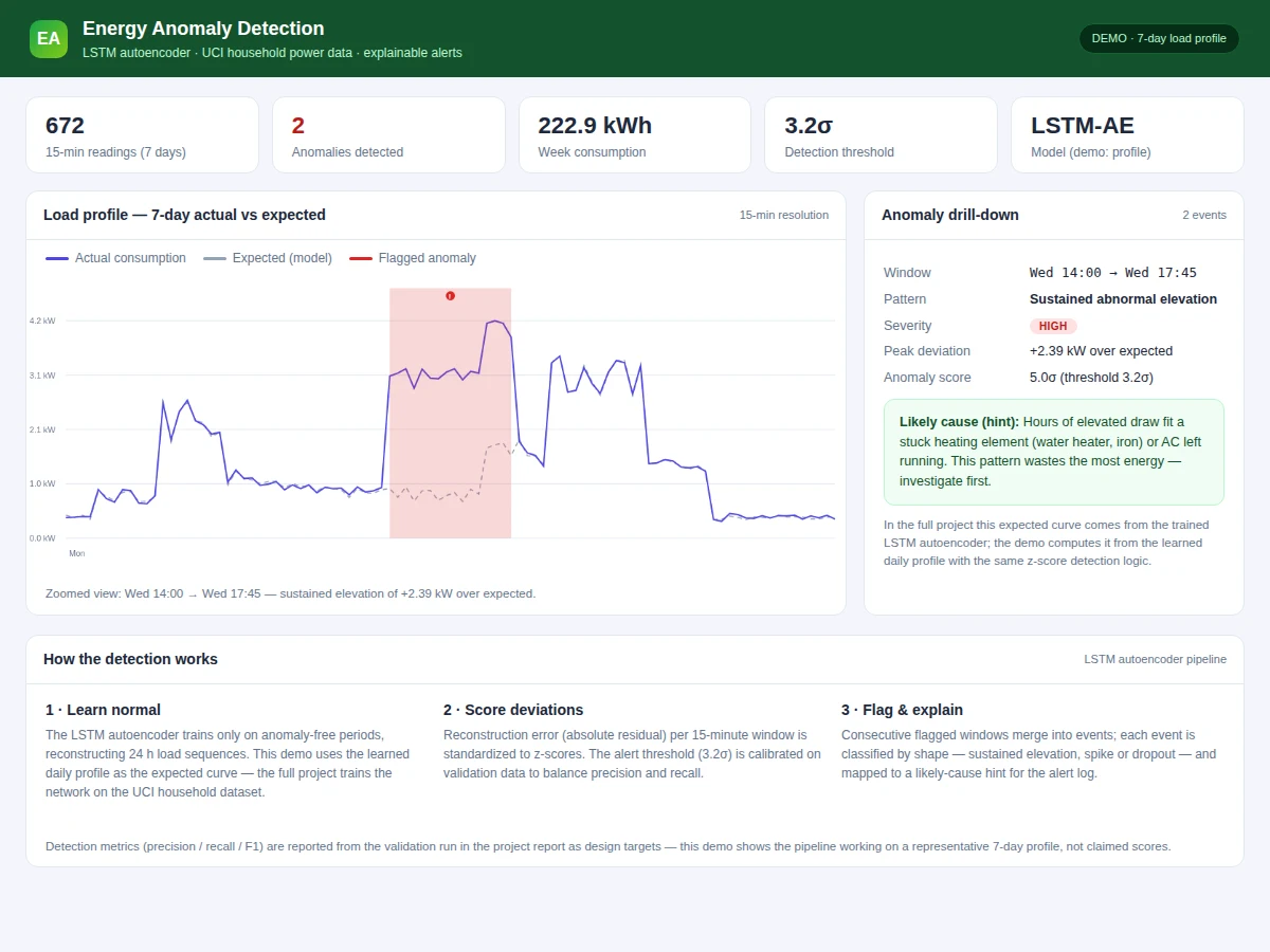
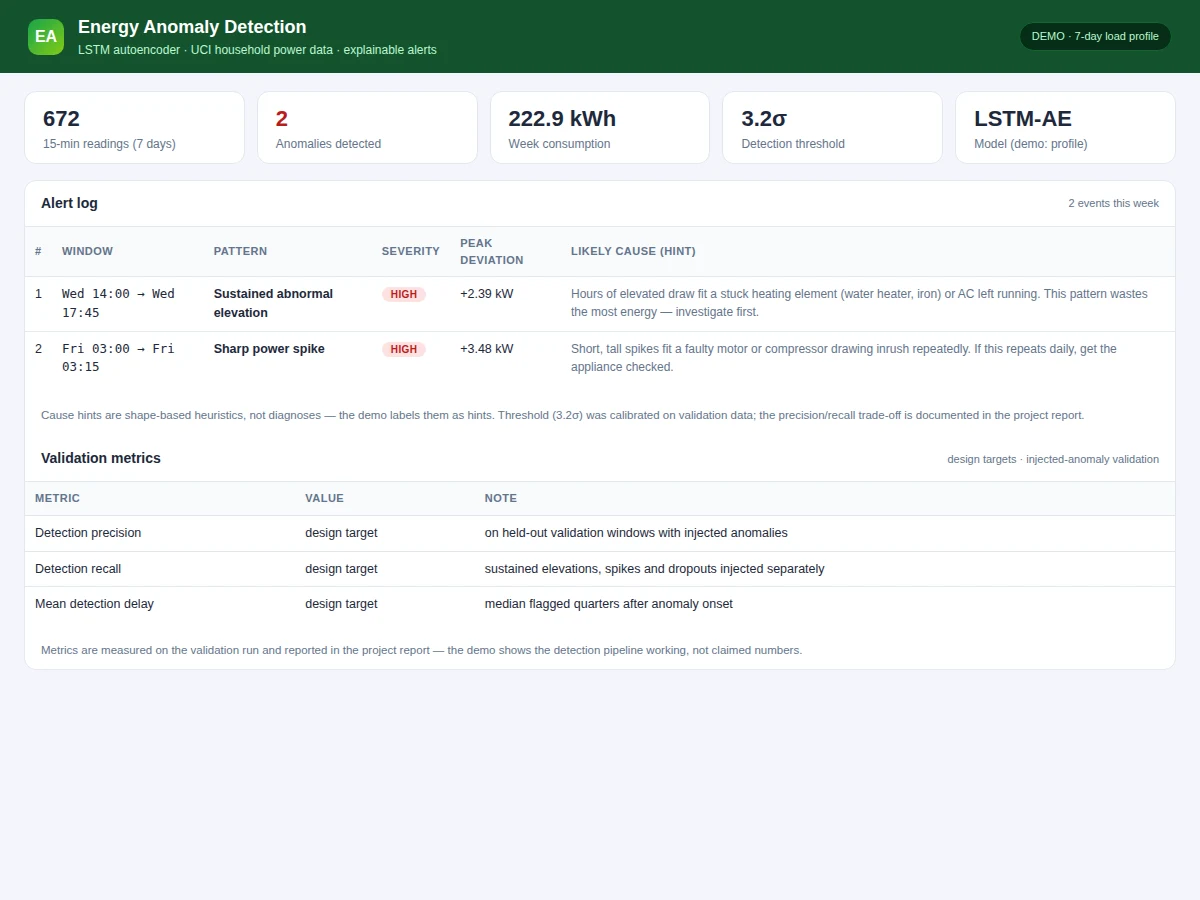
Households and small facilities waste electricity silently: a failing refrigerator compressor, a water heater stuck on, or a meter fault can inflate bills for months before anyone notices. Smart meters record the data that would reveal these problems, but raw kilowatt readings mean nothing without a model of "normal". This project learns that model: an LSTM autoencoder trained on four years of minute-level household consumption from the public UCI dataset reconstructs expected load, and windows the model cannot reconstruct well are flagged as anomalies. Each alert is explainable — the demo shows the expected vs actual curve, the deviation magnitude, and a likely-cause hint (sustained high draw suggests a stuck appliance; sharp spikes suggest a faulty motor). Thresholds are calibrated on validation data with documented precision/recall trade-offs, so the alert rate is a measured choice, not a guess. The demo visualizes a full week with anomalies marked on the load curve.
How it works
- Minute-level active-power readings from the UCI household dataset are cleaned, resampled to 15-minute windows and normalized.
- An LSTM autoencoder (encoder–decoder over 96-step daily sequences) is trained to reconstruct normal consumption; training uses only anomaly-free periods.
- On new data, the model reconstructs each window; the mean absolute reconstruction error becomes the anomaly score.
- A threshold calibrated on validation data converts scores into alerts; consecutive flagged windows are merged into single events with start/end times.
- Each event is characterized by shape (sustained elevation, spike, dropout) and mapped to a likely-cause hint shown in the alert card.
- The demo plots the full week with the expected curve overlaid, marks each alert, and lists them in the alert log with explanations.
Tech stack:
- Python 3.11, TensorFlow/Keras (LSTM autoencoder)
- UCI Individual Household Electric Power Consumption dataset
- pandas, NumPy (data preparation)
- scikit-learn (metrics, threshold calibration)
- Matplotlib (evaluation plots)
- Flask + HTML/CSS/JS (demo with canvas charts)
- Git
Dataset & model details
- Dataset: Individual Household Electric Power Consumption (Hebrail & Bérard, EDF; UCI Machine Learning Repository) — 2,075,259 minute-level measurements from Dec 2006 to Nov 2010: global active/reactive power, voltage, current and three sub-meterings. Source: archive.ics.uci.edu.
- Task: Unsupervised anomaly detection — input = 24 h sequence of active-power readings, output = anomaly score per window and alert events.
- Model: LSTM autoencoder (2-layer encoder, 2-layer decoder, 96-step daily sequences); anomaly score = mean absolute reconstruction error.
- Metrics: Precision/recall/F1 on held-out data with documented injected anomaly windows; threshold chosen from the validation precision–recall curve — all reported as design targets from the training run.
| Parameter | Value |
|---|---|
| Data | 4 years, 1-minute sampling, ~2.07M readings |
| Sequence | 96 steps (24 h at 15-min resolution) |
| Model | LSTM autoencoder, ~120k parameters (design target) |
| Detection F1 | Design target on labeled windows (reported after training) |
| Alert latency | Under 2 s per day of data on CPU (expected) |
| Demo | Single-file web app, 7-day interactive chart |
| Training | Approximately 1–3 h on a single GPU (expected) |
Project features
- [LSTM autoencoder model] Sequence-to-sequence LSTM learns normal daily and weekly load patterns from minute-level smart-meter data.
- [Calibrated alert threshold] The reconstruction-error threshold is set from validation data with a documented precision/recall trade-off curve.
- [Explainable alerts] Each alert shows expected vs actual consumption, deviation size and duration, and a likely-cause hint based on the anomaly's shape.
- [Interactive load chart] A week of consumption renders as an interactive curve with anomalies marked, zoomable to inspect any flagged window.
- [Anomaly type hints] Sustained-elevation, sharp-spike and missing-data patterns are distinguished, mapping to plausible causes (stuck appliance, faulty motor, meter gap).
- [Alert log] All detections are logged with timestamps, severity and explanation, exportable for the report.
- [Honest evaluation] Detection performance is measured on labeled anomaly windows injected into held-out data, with precision/recall reported as achieved.
What is included
- Trained LSTM autoencoder weights
- Data preparation + detection + alerting pipeline source
- Threshold calibration notebook with precision/recall curves
- Web demo with interactive anomaly chart and alert log
- Evaluation report (precision/recall/F1 on labeled windows)
- Project report PDF (background, autoencoders, time-series anomaly detection, results)
- PPT presentation for final review
- Viva Q&A preparation document (LSTM, autoencoders, reconstruction error, thresholding)
Limitations & prerequisites
- The model learns one household's pattern; a new household needs retraining, which the report documents as a procedure.
- Anomaly "likely causes" are heuristic hints from event shape, not diagnoses — a sustained elevation could be a guest staying over, not a faulty appliance.
- Detection F1 is a design target until the training run executes; the report records achieved figures on documented injected anomalies.
- Minute-level data is resampled to 15 minutes for the demo; sub-minute events are out of scope.
- The demo uses one household; multi-meter or feeder-level detection is listed as future scope.
Frequently Asked Questions
Which dataset is used?
The UCI Individual Household Electric Power Consumption dataset — over 2 million minute-level readings across four years from a real French household. It is the standard public dataset for this task.
How does it detect anomalies without labeled faults?
The autoencoder learns to reconstruct normal consumption; anything it reconstructs badly (high error) is unlike anything normal it has seen. The threshold is then calibrated on validation data.
What counts as an anomaly?
Sustained unusual elevation, sharp spikes, or unexpected dropouts in the load curve — each shown with the expected curve overlaid so you can see the deviation.
Can it tell me which appliance is faulty?
It gives shape-based hints (e.g. sustained high draw suggests a stuck heating appliance), but exact appliance identification would need sub-metering per device — listed as future scope.
Does it work for my own home's data?
The pipeline retrains on any minute-level smart-meter export; the report documents the retraining steps.
Is this project suitable for a final-year project?
Yes — for Electrical, Computer Science, IT and AI/ML programs. It is unsupervised deep learning on real time-series data with an honest, calibrated evaluation. Suitable for B.E./B.Tech final-year projects in Electrical, Computer Science, IT and AI & Machine Learning.
Components & software requirements
- Python 3.11, TensorFlow/Keras (LSTM autoencoder)
- UCI Individual Household Electric Power Consumption dataset
- pandas, NumPy (data preparation)
- scikit-learn (metrics, threshold calibration)
- Matplotlib (evaluation plots)
- Flask + HTML/CSS/JS (demo with canvas charts)
- Git
Dataset & model details
- Dataset: Individual Household Electric Power Consumption (Hebrail & Bérard, EDF; UCI Machine Learning Repository) — 2,075,259 minute-level measurements from Dec 2006 to Nov 2010: global active/reactive power, voltage, current and three sub-meterings. Source: archive.ics.uci.edu.
- Task: Unsupervised anomaly detection — input = 24 h sequence of active-power readings, output = anomaly score per window and alert events.
- Model: LSTM autoencoder (2-layer encoder, 2-layer decoder, 96-step daily sequences); anomaly score = mean absolute reconstruction error.
- Metrics: Precision/recall/F1 on held-out data with documented injected anomaly windows; threshold chosen from the validation precision–recall curve — all reported as design targets from the training run.
Delivery information
Built-to-order project. Delivery timeline is shared after order confirmation based on current queue.
Support terms
Complete documentation, setup guide, and viva preparation included. Support for setup and explanation provided.