
More project photos (2)
The problem
Air quality advisories in Indian cities are usually reactive: the AQI number published today describes air people already breathed. Municipal bodies, schools and citizens would all act differently with a reliable 24–48 hour heads-up — rescheduling outdoor activity, issuing health advisories, or planning construction curbs before a severe episode rather than during it. Forecasting AQI is a natural time-series problem because pollution has strong structure: daily traffic cycles, weekly patterns, seasonal stubble-burning and winter inversion episodes all repeat. Yet most student forecasting demos use synthetic or toy CSVs with no connection to real monitoring infrastructure. This project closes that gap: it pulls genuine hourly station data from the OpenAQ platform, computes AQI the standard way from pollutant breakpoints, and trains three real forecasting approaches — statistical (SARIMA), decomposable (Prophet) and deep (LSTM) — on a strict chronological split, comparing them honestly on the same holdout period.
How it works
- The fetch notebook queries the OpenAQ API v3 for hourly PM2.5, PM10, NO2 and O3 at the chosen station over a multi-month window and stores the raw record as CSV.
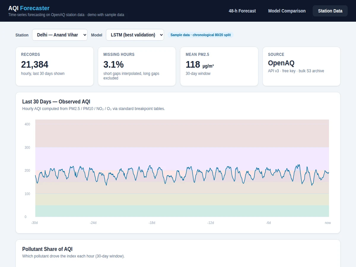
- Raw readings are resampled to a regular hourly index; gaps are flagged, short gaps interpolated by documented rules, and long gaps left missing so the models never train on fabricated stretches.
- Each hour's AQI is computed from the pollutant concentrations using the standard breakpoint tables, and the dominant pollutant for that hour is recorded.
- The series is split chronologically — the first 80% for training, the last 20% as the holdout — with no shuffling, so every model is evaluated only on future it never saw.
- SARIMA is fit on the AQI series with seasonal daily/weekly orders selected by AIC; Prophet is fit with daily and weekly seasonality plus known high-pollution event regressors; the LSTM trains on sliding 72-hour input windows to predict the next 24 hours.
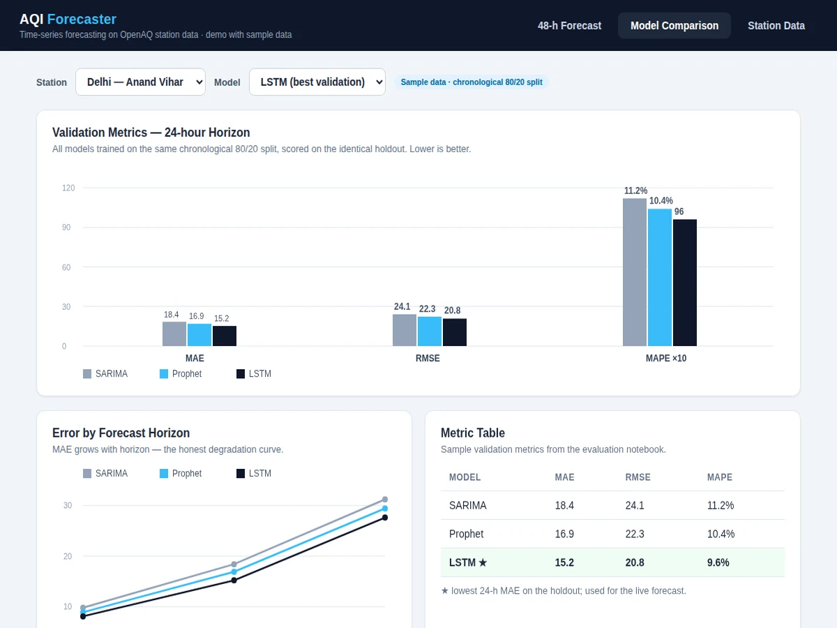
- All three models forecast the holdout period at 6, 24 and 48-hour horizons and are scored with MAE, RMSE and MAPE; residual and error-by-horizon plots go into the report.
- The best-validation model (or a simple average ensemble, configurable) generates the live 48-hour forecast shown on the dashboard with AQI category bands.
Tech stack:
- Python 3.10, pandas and NumPy for time-series wrangling
- OpenAQ API v3 (free key) and bulk S3 archive for station data
- statsmodels (SARIMA fitting and diagnostics)
- Prophet (trend/seasonality decomposition)
- TensorFlow/Keras LSTM for sequence forecasting
- scikit-learn (metrics, chronological splitting utilities)
- Matplotlib (forecast plots, residual diagnostics, error-by-horizon)
- Flask dashboard with 48-hour forecast and model metric cards
| Parameter | Value |
|---|---|
| Data source | OpenAQ platform: hourly PM2.5, PM10, NO2, O3 from a real monitoring station (default Delhi; configurable) |
| Target variable | Hourly AQI computed via standard breakpoint tables; dominant pollutant tracked |
| Models | SARIMA (statsmodels), Prophet, LSTM (TensorFlow/Keras) on identical chronological splits |
| Split protocol | Chronological 80/20 train/holdout; no shuffling; horizons 6 h, 24 h, 48 h |
| Metrics | MAE, RMSE, MAPE per model per horizon — computed by the notebook on your holdout during your build |
| Forecast output | 48-hour AQI forecast with category bands and dominant pollutant |
| Dashboard | Flask app: forecast chart, model comparison cards, station/data info |
| API requirement | Free OpenAQ API key (or bulk S3 download); documented in the setup guide |
Project features
- [Real station data via OpenAQ] Hourly PM2.5, PM10, NO2 and O3 readings are fetched for a genuine monitoring station (default: a Delhi station) through the OpenAQ API v3 with a free key, or from its bulk S3 archive — no synthetic CSVs anywhere in the pipeline.
- [Standard AQI computation] Pollutant concentrations are converted to AQI using official breakpoint tables (US EPA method), with the dominant pollutant identified per hour, so the target variable is defined exactly the way published AQI numbers are.
- [Three-model comparison] SARIMA (statistical baseline), Prophet (trend plus daily/weekly seasonality with holiday effects) and an LSTM network (sequence learning on lagged windows) are trained on the same chronological 80/20 split and compared on identical holdout data.
- [Honest evaluation protocol] The split is strictly chronological — no shuffling, no leakage from the future — and every model is scored on MAE, RMSE and MAPE over multiple forecast horizons (6 h, 24 h, 48 h) so degradation with horizon is visible, not hidden.
- [48-hour forecast dashboard] A web dashboard plots the next 48 hours of predicted AQI with category color bands (Good through Severe), the dominant pollutant, and per-model metric cards from the validation run.
- [Missing-data handling] Station gaps — a reality of real monitoring networks — are handled with documented resampling and interpolation rules, and the report quantifies how much of the raw record was missing.
- [Retrainable pipeline] Changing the city or station is a configuration change: the fetch, AQI computation, training and evaluation notebooks rerun end to end for any OpenAQ station with sufficient history.
What is included
- Complete source code (fetch, preprocessing, AQI computation, three training pipelines, evaluation, dashboard)
- Jupyter notebooks for data fetch, EDA, model training and evaluation (buyer-run: fetch your station's data, train, evaluate)
- Sample fetched dataset snapshot so the pipeline runs even before a fresh API pull
- Project report PDF (background, data audit, methodology per model, evaluation tables, error analysis, limitations)
- PPT presentation for final review
- Viva Q&A preparation document (stationarity, ARIMA orders, Prophet components, LSTM windows, leakage, metrics)
- Setup guide (Python environment, OpenAQ free API key, running the pipeline, reading the dashboard)
Limitations & prerequisites
- Forecast skill degrades with horizon: 6-hour forecasts track the series closely while 48-hour forecasts smooth toward the seasonal mean — the report shows error-by-horizon curves instead of quoting a single flattering number.
- The model learns one station's history: it does not transfer to another city without retraining, and extreme episodes (crop-burning spikes, dust storms) are poorly captured because they are rare in the training record.
- Real station data has gaps from maintenance and outages; long missing stretches are excluded rather than invented, which shortens the usable history at some stations.
- No performance number is pre-claimed: MAE, RMSE and MAPE are computed by the evaluation notebook on your holdout during your build, and the report presents them with the horizon breakdown.
- OpenAQ historical coverage varies by station and period; the setup guide shows how to check a station's available range before committing to it, and the free API key has rate limits the fetch notebook respects.
Frequently Asked Questions
Is this project suitable for a final-year project?
Yes — it fits Computer Science, AI/ML and Data Science programs and gives examiners a complete applied ML story: real data sourcing, time-series methodology, three-model comparison, honest evaluation and a working dashboard.
Which dataset is used?
Hourly pollutant measurements (PM2.5, PM10, NO2, O3) from the OpenAQ platform — a real global monitoring-data aggregator — for a chosen station (default: a Delhi station). AQI is computed from the concentrations using standard breakpoint tables, and the notebooks document the station, period and missing-data share.
Which models are used and how are they compared?
SARIMA (statsmodels), Prophet and an LSTM (TensorFlow/Keras), all trained on the same chronological 80/20 split and scored on MAE, RMSE and MAPE at 6, 24 and 48-hour horizons on the holdout the models never saw.
Is the forecast accuracy guaranteed?
No — and any listing that guarantees it is inventing numbers. The evaluation notebook computes MAE, RMSE and MAPE on your holdout during your build; the report presents them per horizon, including how error grows at 48 hours.
Can I change the city?
Yes — the station is a configuration value. The fetch, AQI, training and evaluation notebooks rerun end to end for any OpenAQ station with enough hourly history; the setup guide shows how to check coverage first.
What will I receive with the project?
Full source code and notebooks, a sample dataset snapshot, the project report PDF, PPT, viva Q&A document and the setup guide covering the environment, the free OpenAQ API key and the dashboard. Suitable for B.E./B.Tech final-year projects in Computer Science, AI/ML and Data Science.
Components & software requirements
- Python 3.10, pandas and NumPy for time-series wrangling
- OpenAQ API v3 (free key) and bulk S3 archive for station data
- statsmodels (SARIMA fitting and diagnostics)
- Prophet (trend/seasonality decomposition)
- TensorFlow/Keras LSTM for sequence forecasting
- scikit-learn (metrics, chronological splitting utilities)
- Matplotlib (forecast plots, residual diagnostics, error-by-horizon)
- Flask dashboard with 48-hour forecast and model metric cards
Delivery information
Built-to-order project. Delivery timeline is shared after order confirmation based on current queue.
Support terms
Complete documentation, setup guide, and viva preparation included. Support for setup and explanation provided.