
More project photos (2)
The problem
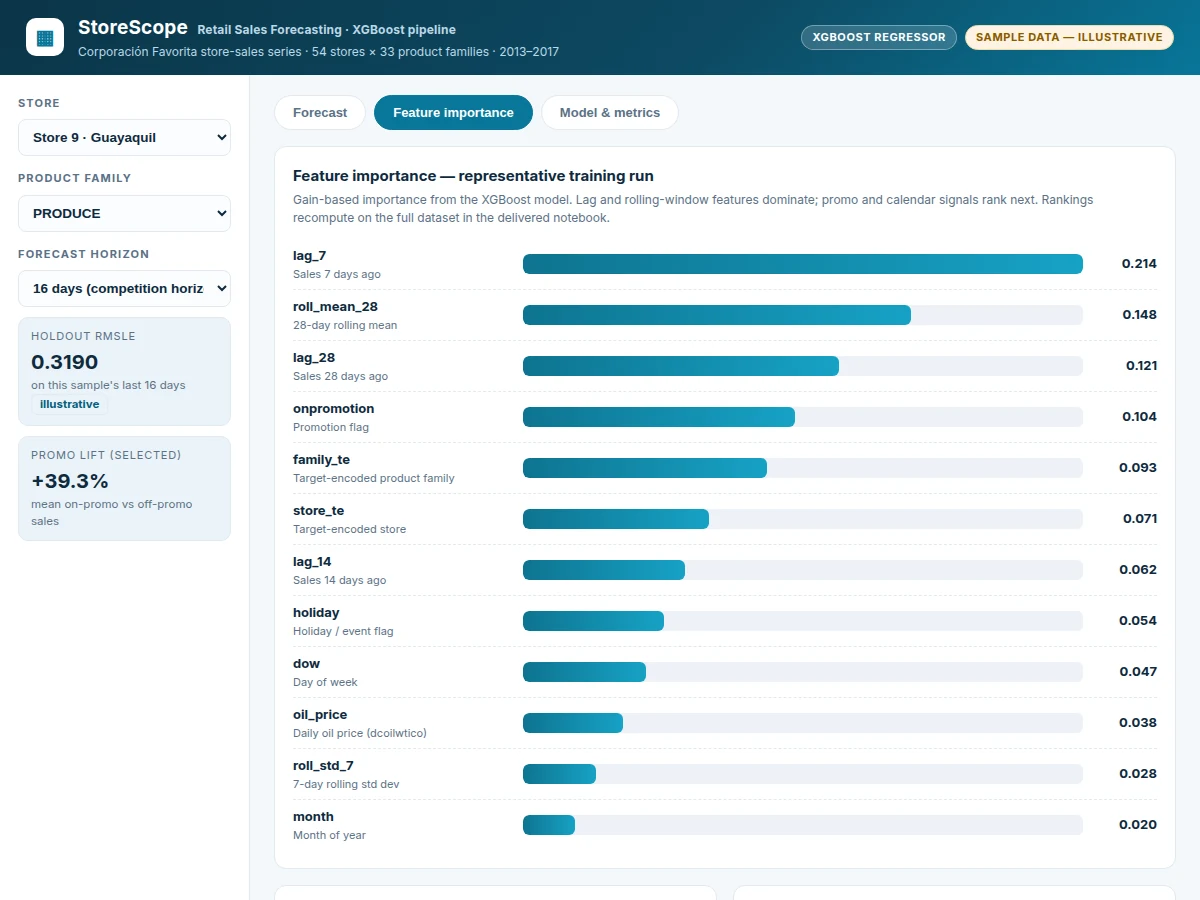
Retailers lose money on both sides of a bad forecast: overstock ties up cash and expires, stockouts lose sales. Classical tools — moving averages, Holt-Winters, per-series ARIMA — need separate tuning for every demand series and cannot consume promotion flags, holiday calendars or oil prices as regressors without heavy extensions. This project takes the competition-validated route instead: one global XGBoost regressor trained over engineered features for all 1,782 store × product-family series of the Corporación Favorita dataset (54 stores, 33 families, 2013–2017). The pipeline builds leakage-safe lag (7/14/28 days) and rolling-window features, onpromotion flags, holiday/event calendar signals, target-encoded store and family identifiers and the daily oil price; trains on log1p-transformed sales with early stopping; and validates with three walk-forward folds scored by RMSLE — the competition's official metric. A Flask dashboard renders forecast-vs-actual charts with 16-day prediction bands, gain-based feature-importance rankings and promotion-lift estimates per family.
Favorita dataset: 54 stores, 33 families, about 3M training rows.
Follow the working sequence
How it works
- The five source tables (daily sales, store metadata, promotions, holidays/events, oil prices) load from the Corporación Favorita dataset and align on (date, store, family): 54 stores × 33 product families, about 1,782 series and roughly 3.0 million training rows from 2013-01-01 to 2017-08-15.
- Each series is reindexed to a continuous daily grid so every calendar day is represented; the competition convention treats missing days as zero-sales days.
- The feature builder shifts every lag and rolling statistic backwards (lags of 7, 14 and 28 days; rolling means and standard deviations over 7, 14 and 28-day windows) so no future sale leaks into a training row, then joins calendar, promo, target-encoding and oil-price features onto the same row.
- The target is log1p-transformed to match the RMSLE objective; the XGBoost regressor trains globally with early stopping, so the tree count is selected by validation RMSLE rather than fixed in advance.
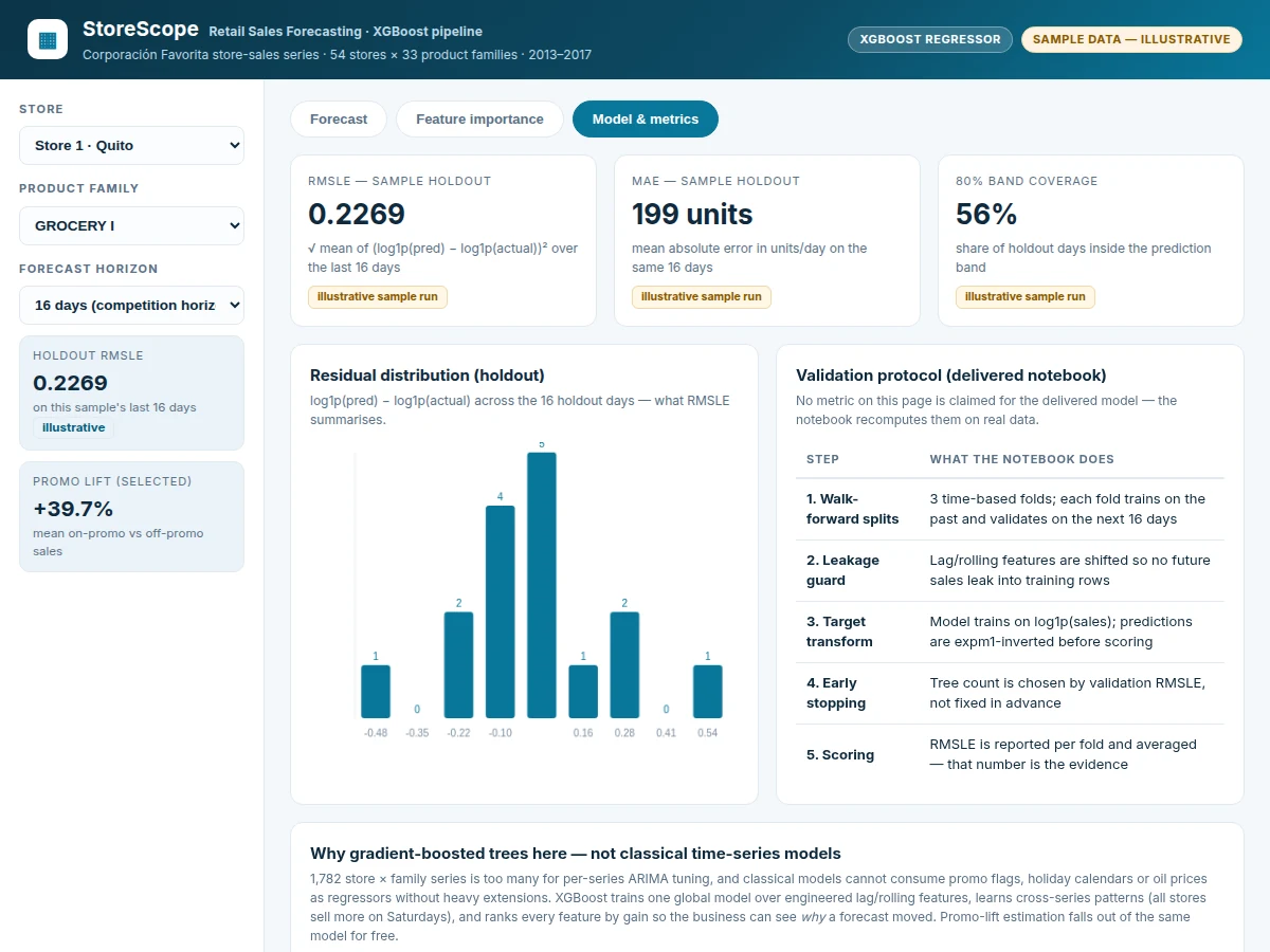
- Walk-forward validation scores three folds: train on the past, predict the next 16 days, report RMSLE per fold and the mean across folds.
- Predictions are expm1-inverted back to original units; the dashboard renders the 16-day forecast with its 80% band, the feature-importance ranking and the promo-lift table.
- New dated sales data flows through the same notebook — re-run ingestion, features and training, and the dashboard reads the refreshed forecast file.
Tech stack:
- Python 3.10, pandas, NumPy — data wrangling and feature engineering
- XGBoost regressor on log1p(sales), with early stopping on the validation fold
- scikit-learn — walk-forward splits, target encoders, RMSLE scoring
- Jupyter Notebook — the documented end-to-end training pipeline
- Flask + HTML5, CSS3, JavaScript — the three-view forecast dashboard
- Matplotlib, Seaborn — exploratory analysis and validation plots
Dataset & model details
- Dataset: Store Sales — Time Series Forecasting (Kaggle competition)
- Source: Kaggle; daily unit-sales data from Corporación Favorita, a large Ecuadorian grocery retailer
- Task: Regression — predict daily unit sales (the
salescolumn) at (date × store × family) granularity - Scale: 54 stores × 33 product families (≈1,782 series); train 2013-01-01 to 2017-08-15 (≈3.0M rows); 16-day test horizon
- Columns used: sales (target), onpromotion flags, store metadata, holidays/events calendar, daily oil price (dcoilwtico)
- Model: XGBoost regressor
- Input: ≈30 engineered features per row — lags 7/14/28, rolling means/std over 7/14/28-day windows, onpromotion, holiday/event flags, day-of-week, month, target-encoded store and family means, oil price
- Prediction task: daily unit sales for the next 16 days per store × family
- Output: point forecast in units/day (expm1-inverted) plus an 80% prediction band in the dashboard
- Evaluation: RMSLE — sqrt(mean((log1p(pred) − log1p(actual))²)) — the competition's official metric, reported per walk-forward fold and averaged. No RMSLE value is pre-claimed; the notebook computes it on the student's own splits.
| Parameter | Value |
|---|---|
| Series modelled | 54 stores × 33 product families (≈1,782 series) |
| Training window | 2013-01-01 to 2017-08-15 (public Kaggle dataset) |
| Training rows | ≈3.0 million (design target on the full download) |
| Target | Daily unit sales per store × product family |
| Forecast horizon | 16 days ahead (design target, matching the competition) |
| Engineered features | ≈30 per training row |
| Validation | 3 walk-forward folds, 16-day holdout each (design target) |
| Metric | RMSLE (Root Mean Squared Logarithmic Error) |
| Model | XGBoost regressor on log1p(sales), early stopping on validation (design target) |
| Dashboard | Flask + JavaScript charts, 3 views: forecast, feature importance, metrics (delivered) |
| Training time | Hardware-dependent (expected); a sampled-subset mode is included for quick iteration |
Project features
- [Engineered time-series feature pipeline] Every (date × store × family) point becomes a supervised-learning row: lags 7/14/28, rolling means and standard deviations over 7/14/28-day windows, onpromotion flags, holiday/event calendar, day-of-week and month encodings, target-encoded store and family identifiers, and the daily oil price — each lag shifted so no future sale leaks into training.
- [XGBoost regression model] A single global gradient-boosted regressor trains on log1p-transformed daily unit sales, so one model learns patterns shared across all 1,782 series (for example weekend uplift) instead of fitting thousands of fragile per-series models. The tree count is chosen by early stopping on the validation fold.
- [Walk-forward validation] The model is scored on three time-based folds — each fold trains on the past and validates on the next 16 days, mirroring the competition horizon — reporting RMSLE per fold and the mean. The measured RMSLE on the student's own splits is the project's evidence; no accuracy is pre-claimed.
- [Forecast-vs-actual dashboard] The Flask dashboard draws 90 days of history with the 16-day forecast band, promotion-day markers and a day-by-day forecast table with 80% prediction bands for any store × family selection.
- [Feature-importance analysis] Gain-based importance rankings show which engineered features drive the forecasts — lags and rolling statistics rank first, followed by promotion and calendar signals — so the student can explain why a forecast moved.
- [Promo-lift estimation] On-promotion versus off-promotion average sales are compared per product family to quantify promotion uplift — the business insight the promo flag lets the model learn.
- [Configurable horizon and retraining] (Configurable) The forecast horizon and the store/family subset are parameters in the notebook; retraining on new dated sales data is a single notebook re-run. No online learning is implemented.
- [Documented Jupyter notebook] The full pipeline — exploratory analysis, feature engineering, training, validation and plots — ships as a commented notebook the student can run, modify and defend in the viva.
What is included
- Documented Jupyter notebook: exploratory analysis, feature engineering, XGBoost training, walk-forward validation, RMSLE scoring and all plots
- Flask forecast dashboard (forecast, feature-importance and metrics views) with the working demo as reference
- Project report PDF (dataset, feature design, validation protocol, results discussion)
- PPT presentation for final review
- Viva Q&A preparation document (gradient boosting, leakage in time-series features, RMSLE vs RMSE, target encoding, early stopping)
- Setup guide: dataset download, environment setup, running the notebook, demo walkthrough
Limitations & prerequisites
- No accuracy is pre-claimed: the RMSLE the student reports must be measured by the notebook on their own walk-forward splits, and it varies with the data subset, feature choices and hyperparameters.
- The public dataset ends in August 2017 — it demonstrates the method on real retail data, but a buyer wanting current local retail data must supply their own dated daily-sales series.
- Forecasts assume the future resembles the past: unprecedented promotions, brand-new stores with no sales history, or regime changes degrade accuracy; cold-start series have no lag features to draw on.
- The model does not learn online; retraining on new data is a manual notebook re-run.
- Prediction bands in the demo dashboard are illustrative fixed-width bands; the delivered notebook computes band coverage on the student's own holdout.
- Full-dataset training needs about 8 GB RAM (expected); the sampled-subset mode is provided for lighter machines.
Frequently Asked Questions
Which dataset and model does this project use?
The Kaggle "Store Sales — Time Series Forecasting" dataset from Corporación Favorita: daily unit sales across 54 stores and 33 product families from 2013 to 2017, with promotion flags, a holiday calendar and oil prices. The model is an XGBoost regressor trained on log1p-transformed sales with engineered lag, rolling, promo, calendar and target-encoding features, validated with walk-forward splits.
Is the accuracy guaranteed?
No accuracy number is pre-claimed. The delivered notebook computes RMSLE on the student's own walk-forward holdout folds, and that measured number is the project's evidence. It varies with the data subset used, the feature choices and the hyperparameters — the report documents the protocol so the result is reproducible and defensible.
How is this different from ARIMA or Holt-Winters forecasting?
Classical models are fitted per series, need separate tuning for each of the 1,782 series, and cannot consume promotion flags, holiday calendars or oil prices as regressors without heavy extensions. One global XGBoost model trains over engineered features across all series, learns shared patterns like weekend uplift, and ranks every feature by gain.
Can it work on a retailer's own sales data?
Yes, if the data has dated daily sales per product or store. The notebook's ingestion step is documented for swapping in a custom CSV with the same columns (date, store, family, sales, onpromotion), after which feature engineering, training and the dashboard run unchanged. Very sparse or short sales histories will forecast less reliably than the full dataset.
Is this project suitable for a final-year project?
Yes — for Computer Science, AI/ML and Data Science programs. It demonstrates time-series feature engineering, gradient-boosted regression, leakage-safe walk-forward validation, the RMSLE metric, and a business-readable dashboard with feature-importance and promo-lift analysis — a complete, defensible end-to-end ML workflow with clear business reporting.
Components & software requirements
- Python 3.10, pandas, NumPy — data wrangling and feature engineering
- XGBoost regressor on log1p(sales), with early stopping on the validation fold
- scikit-learn — walk-forward splits, target encoders, RMSLE scoring
- Jupyter Notebook — the documented end-to-end training pipeline
- Flask + HTML5, CSS3, JavaScript — the three-view forecast dashboard
- Matplotlib, Seaborn — exploratory analysis and validation plots
Dataset & model details
- Dataset: Store Sales — Time Series Forecasting (Kaggle competition)
- Source: Kaggle; daily unit-sales data from Corporación Favorita, a large Ecuadorian grocery retailer
- Task: Regression — predict daily unit sales (the
salescolumn) at (date × store × family) granularity - Scale: 54 stores × 33 product families (≈1,782 series); train 2013-01-01 to 2017-08-15 (≈3.0M rows); 16-day test horizon
- Columns used: sales (target), onpromotion flags, store metadata, holidays/events calendar, daily oil price (dcoilwtico)
- Model: XGBoost regressor
- Input: ≈30 engineered features per row — lags 7/14/28, rolling means/std over 7/14/28-day windows, onpromotion, holiday/event flags, day-of-week, month, target-encoded store and family means, oil price
- Prediction task: daily unit sales for the next 16 days per store × family
- Output: point forecast in units/day (expm1-inverted) plus an 80% prediction band in the dashboard
- Evaluation: RMSLE — sqrt(mean((log1p(pred) − log1p(actual))²)) — the competition's official metric, reported per walk-forward fold and averaged. No RMSLE value is pre-claimed; the notebook computes it on the student's own splits.
Delivery information
Built-to-order project. Delivery timeline is shared after order confirmation based on current queue.
Support terms
Complete documentation, setup guide, and viva preparation included. Support for setup and explanation provided.
Download free synopsis (PDF)
Enter your name and email — the synopsis PDF downloads immediately. We may send occasional project updates; no spam, unsubscribe anytime.