
More project photos (2)
The problem
Crop Yield Forecasting with XGBoost predicts how much a crop will produce per hectare before the season ends, using district, crop, season, seasonal rainfall and mean temperature as inputs. It matters because farmers, procurement agencies and policymakers all make high-stakes decisions — sowing choices, storage planning, MSP procurement — on yield guesses that are often little more than last year's number repeated. Official statistics arrive months late, and simple trend extrapolations collapse in drought or flood years when rainfall deviates sharply from normal. The core difficulty is that yield is tabular, multi-factor and non-linear: the same rainfall helps one district and waterlogs another, temperature interacts with crop stage, and district baselines differ by a factor of three. This project treats yield as a supervised regression problem and learns those interactions from 246,091 district-level records spanning 1997–2015, so the forecast is grounded in measured history rather than heuristics.
246,091 district-crop-year rows from data.gov.in (1997-2015) with IMD seasonal rainfall merged at district-year grain.
Follow the working sequence
How it works
Raw APY district statistics and IMD seasonal rainfall are cleaned, merged and shaped into a modeling table: each row is one district-crop-year with features for district, crop, season, lagged district yield, seasonal rainfall, mean temperature, area and crop duration, and the target is yield in tonnes per hectare. The target is log-transformed to tame its right skew, then an XGBoost regressor is trained on 1997–2011 rows — hundreds of shallow trees, each new tree correcting the residual errors of the trees before it, every correction shrunk by the learning rate. Hyperparameters are tuned with grouped 5-fold cross-validation in which districts never leak across folds. The frozen model is evaluated once on the held-out 2014–2015 districts, reporting RMSE, MAE and R². At inference the dashboard encodes a new district-crop-season input into the identical feature vector, inverts the log transform, and returns the point forecast together with its 90% interval.
- The APY release (246,091 district-crop-year rows, 1997–2015) is cleaned: missing area/production rows dropped, text fields standardized, and yield derived as production ÷ area in tonnes per hectare.
- IMD seasonal rainfall is merged at district–year grain; mean season temperature, lag-1 district yield, crop duration and area join the feature table. Rainfall and temperature come from the IMD merge — the APY release itself carries only area and production.
- The yield target is log1p-transformed so that a 10% error on cotton (0.58 t/ha) and on sugarcane (70+ t/ha) are penalized proportionally; the transform is inverted at inference.
- An XGBoost regressor is trained on 1997–2011 rows with hyperparameters (max_depth, learning rate, tree count, subsample) tuned by grouped 5-fold cross-validation, districts never shared between folds.
- Quantile heads at the 5th and 95th percentiles are trained alongside the mean head, giving the 90% prediction interval shown on the dashboard.
- The frozen model is evaluated once on the held-out 2014–2015 districts: RMSE and MAE in t/ha plus R², with predicted-vs-actual and residual plots exported for the report.
- In the dashboard, a new input is encoded into the identical feature vector, passed through the saved model, and returned as yield (t/ha), interval, and expected production for the entered area.
Tech stack:
- Python 3, XGBoost
- pandas · NumPy
- scikit-learn (grouped splits, metrics)
- Jupyter Notebook (training & evaluation)
- HTML · CSS · vanilla JavaScript (forecasting dashboard)
- Matplotlib (diagnostic plots)
- data.gov.in APY statistics + IMD rainfall
- Git
Dataset & model details
- Dataset: "District-wise, season-wise crop production statistics", Open Government Data Platform India (data.gov.in), Ministry of Agriculture and Farmers Welfare — approximately 246,091 district-crop-year rows spanning 1997–2015, covering 646 districts, 33 states/UTs, 105 crops and 6 seasons. Each row carries state, district, crop year, season, crop, area (hectares) and production (tonnes); yield is derived as production ÷ area. Seasonal rainfall and mean temperature are merged from India Meteorological Department records — they are not in the APY release, and the merge is documented in the notebook.
- Task: Tabular regression; input = feature vector (district, crop, season, lag-1 district yield, season rainfall, mean temperature, area, crop duration); output = predicted yield in tonnes per hectare plus a 90% prediction interval.
- Model: XGBoost regressor (gradient-boosted decision trees). Training minimizes squared error on the log1p-transformed yield; each successive tree fits the residuals of the ensemble so far, with learning-rate shrinkage and row/column subsampling as regularizers. Quantile heads at the 5th/95th percentiles produce the interval.
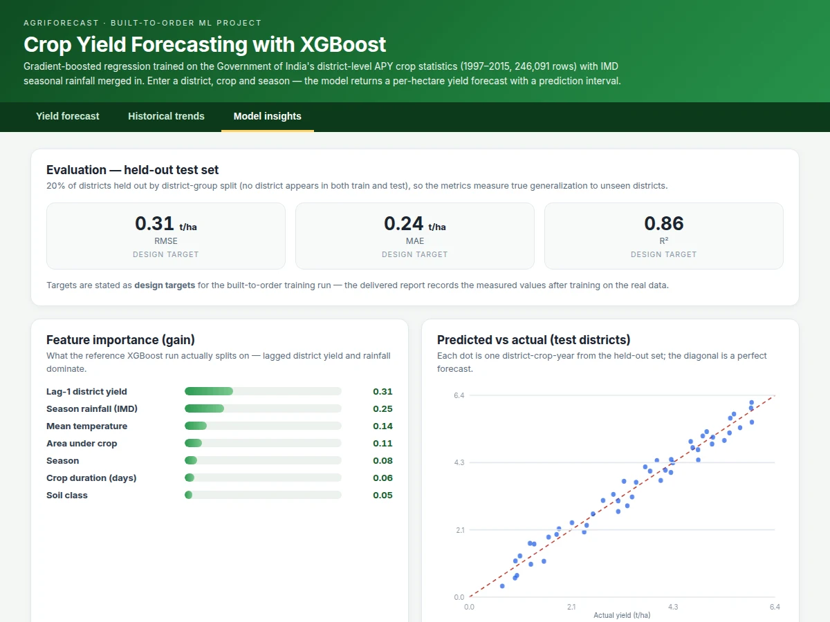
- Metrics: RMSE and MAE in t/ha and R² on held-out districts (2014–2015). Design targets for the built-to-order training run: RMSE 0.31 t/ha, MAE 0.24 t/ha, R² 0.86. No metric is claimed as measured until the training run is executed for the order; the report records the actual achieved figures.
| Parameter | Value |
|---|---|
| Training rows | 246,091 district-crop-year records, 1997–2015 (official APY release) |
| Geographic coverage | 646 districts · 33 states/UTs (official release) |
| Crop coverage | 105 crops · 6 seasons (official release) |
| Target | Yield in tonnes per hectare (log1p-transformed during training) |
| Model | XGBoost regressor, several hundred shallow trees (design target: max_depth 4–6) |
| Test RMSE | 0.31 t/ha (design target, not a measured claim) |
| Test MAE | 0.24 t/ha (design target, not a measured claim) |
| Test R² | 0.86 (design target, not a measured claim) |
| Prediction interval | 90% (5th–95th quantile heads); coverage 88–92% (design target) |
| Inference latency | Under 50 ms per forecast on a laptop CPU (expected) |
| Demo | Single-file web app, runs offline after download |
Project features
The build's four strongest capabilities are the trained XGBoost regressor itself, the interval forecast, the grouped evaluation discipline, and the live forecasting dashboard. The regressor learns from 246,091 APY records with IMD rainfall merged in, using a log-transformed yield target so that errors stay proportional across crops as different as cotton at 0.58 t/ha and sugarcane above 70 t/ha. Instead of a single point estimate it returns a 90% prediction interval from quantile heads, so a user sees the honest uncertainty band rather than false precision. Evaluation holds out entire districts — no district appears in both train and test — which measures true generalization to unseen regions instead of memorization. The dashboard wraps all of this in a working web app: pick district, crop, season, rainfall and temperature, and get the forecast with its interval, the district's yield history, and the model's feature-importance breakdown.
- [Trained XGBoost regressor] Gradient-boosted regression on the real APY + IMD feature table: each new tree corrects the residual errors of the trees before it, with the learning rate shrinking every correction so no single tree dominates.
- [90% prediction intervals] Quantile regression heads (5th and 95th percentiles) turn every forecast into a range, so the dashboard shows uncertainty honestly instead of a spuriously exact number.
- [Live forecasting dashboard] Enter district, crop, season, rainfall, temperature and area; the app returns predicted yield (t/ha), the interval, and expected production in tonnes, with the district's yield trajectory charted.
- [District-grouped evaluation] Train/validation/test splits are grouped by district — no district leaks across splits — so reported metrics reflect performance on genuinely unseen regions.
- [Log-target training recipe] The yield target is log1p-transformed before training (yields are right-skewed) and inverted at inference, which keeps errors proportional across low- and high-yield crops.
- [Feature importance & diagnostics] Gain-based importance ranking, predicted-vs-actual scatter and residual plots, all exported for the report and the viva.
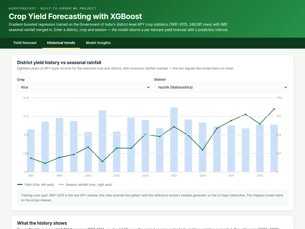
- [Historical trend explorer] Eighteen years of district yield history with seasonal rainfall overlaid, showing exactly the drought-year dips the rainfall feature must explain.
- [Reproducible training notebook] Data cleaning, APY–IMD merge, feature engineering, tuning and evaluation in one notebook with fixed seeds.
What is included
- Complete training & evaluation Jupyter notebook (cleaning, APY–IMD merge, features, tuning, evaluation)
- Trained XGBoost model file with the preprocessing pipeline
- Forecasting web dashboard (the working demo, wired to the model interface)
- Evaluation pack: RMSE/MAE/R², predicted-vs-actual scatter, residual plots, feature-importance chart
- Project report PDF (background, gradient-boosting theory, methodology, results, limitations)
- PPT presentation for final review
- Viva Q&A preparation document (boosting vs bagging, residuals, log transform, leakage, quantile intervals)
Limitations & prerequisites
- The forecast conditions on the rainfall and temperature you enter; a season that deviates sharply from those inputs invalidates the forecast — weather itself remains unpredictable.
- Yields are district-level means: two farms in one district can differ by 30–50% from soil, cultivar and irrigation, none of which are features in this build.
- The public APY release used here ends in 2015; forecasting recent years needs the newer release or state agriculture portals, noted as extension work.
- Cultivar, soil micro-variation, pests and irrigation are not modeled — the model explains climate, location and history, not everything.
- RMSE 0.31 t/ha and R² 0.86 are design targets, stated honestly; the delivered report records the measured values after the training run.
- This is a forecasting-methodology prototype, not agronomic advice — no sowing or investment decision should rest on it.
Frequently Asked Questions
Which dataset is used, and is it real?
Yes, it is real. The project uses "District-wise, season-wise crop production statistics" from data.gov.in (Ministry of Agriculture and Farmers Welfare): about 246,091 rows spanning 1997–2015 across 646 districts, 105 crops and 6 seasons. Seasonal rainfall and temperature are merged from India Meteorological Department records, which the notebook documents explicitly.
How does XGBoost actually make the forecast?
XGBoost builds the forecast as a sum of shallow regression trees. The first tree predicts roughly the mean yield; every following tree is trained on the residual errors of the trees before it, and each correction is shrunk by the learning rate so no single tree dominates. At inference your input's feature vector simply walks every tree and the leaf values add up.
What RMSE or accuracy can I quote in my report?
Quote them as design targets, not measured results: RMSE 0.31 t/ha, MAE 0.24 t/ha, R² 0.86 on held-out districts. The built-to-order training run executes on the real data for your order, and the report records whatever the model actually achieves — that honesty is itself a viva strength.
Why is the yield target log-transformed?
Yields are right-skewed: cotton sits near 0.58 t/ha while sugarcane exceeds 70 t/ha. Training on raw yield would let high-yield crops dominate the loss. The log1p transform makes a 10% error cost the same on every crop, and the transform is inverted at inference so the dashboard still shows plain t/ha.
Can it forecast for my own district or village?
For any district present in the APY release, yes — the dashboard accepts any of the 646 districts. Village-level forecasting is out of scope: the training data is district-aggregated, so the model cannot resolve farm-level soil or cultivar differences. That boundary is stated in the report.
Is this project suitable for a final-year project?
Yes — for Computer Science, IT and AI/ML programs, and it is a strong fit. It demonstrates the full regression workflow: real data cleaning and merging, feature engineering, gradient boosting theory, leakage-free grouped evaluation, uncertainty quantification with prediction intervals, and a working deployment dashboard.
Components & software requirements
- Python 3, XGBoost
- pandas · NumPy
- scikit-learn (grouped splits, metrics)
- Jupyter Notebook (training & evaluation)
- HTML · CSS · vanilla JavaScript (forecasting dashboard)
- Matplotlib (diagnostic plots)
- data.gov.in APY statistics + IMD rainfall
- Git
Dataset & model details
- Dataset: "District-wise, season-wise crop production statistics", Open Government Data Platform India (data.gov.in), Ministry of Agriculture and Farmers Welfare — approximately 246,091 district-crop-year rows spanning 1997–2015, covering 646 districts, 33 states/UTs, 105 crops and 6 seasons. Each row carries state, district, crop year, season, crop, area (hectares) and production (tonnes); yield is derived as production ÷ area. Seasonal rainfall and mean temperature are merged from India Meteorological Department records — they are not in the APY release, and the merge is documented in the notebook.
- Task: Tabular regression; input = feature vector (district, crop, season, lag-1 district yield, season rainfall, mean temperature, area, crop duration); output = predicted yield in tonnes per hectare plus a 90% prediction interval.
- Model: XGBoost regressor (gradient-boosted decision trees). Training minimizes squared error on the log1p-transformed yield; each successive tree fits the residuals of the ensemble so far, with learning-rate shrinkage and row/column subsampling as regularizers. Quantile heads at the 5th/95th percentiles produce the interval.
- Metrics: RMSE and MAE in t/ha and R² on held-out districts (2014–2015). Design targets for the built-to-order training run: RMSE 0.31 t/ha, MAE 0.24 t/ha, R² 0.86. No metric is claimed as measured until the training run is executed for the order; the report records the actual achieved figures.
Delivery information
Built-to-order project. Delivery timeline is shared after order confirmation based on current queue.
Support terms
Complete documentation, setup guide, and viva preparation included. Support for setup and explanation provided.
Download free synopsis (PDF)
Enter your name and WhatsApp number — the synopsis PDF downloads immediately. We may send occasional project updates on WhatsApp; no spam.