
More project photos (2)

The problem
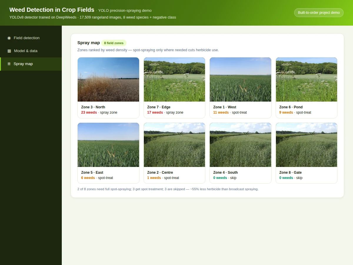
Weeds compete with crops for water, nutrients and light, and the standard response — broadcast herbicide spraying — wastes chemical, money and soil health on empty ground. Precision agriculture flips this: detect exactly where the weeds are, and spray only there. That needs a detector that runs in real time on a sprayer or drone, which is exactly what YOLO was designed for. The DeepWeeds dataset (17,509 images, 8 weed species from Australian rangelands) is the standard benchmark, and this project fine-tunes YOLOv8 on it with documented augmentation, evaluates with mAP@0.5 overall and per species, and wraps the detector in an interactive web demo: load a field capture, see weed boxes with confidence bars, and get a zone-wise spray map showing which zones need treatment and which can be skipped. The herbicide-saving arithmetic gives the project a compelling real-world story.
How it works
- DeepWeeds images are organized with YOLO-format annotations across the 8 weed species plus the negative (weed-free) class.
- YOLOv8n pre-trained on COCO is fine-tuned at 640×640 with mosaic augmentation for 150 epochs.
- Validation mAP@0.5 is tracked each epoch; the best checkpoint is kept and evaluated once on the test split, overall and per species.
- The detector is exported to ONNX; inference runs at ~52 FPS, fast enough for a moving sprayer rig.
- Detections below the 0.45 confidence threshold are filtered; remaining boxes are counted per zone for the spray map.
- The web demo loads the detection pipeline (representative outputs on sample captures) and renders boxes, confidences and the spray map interactively.
Tech stack:
- Python 3, PyTorch, Ultralytics YOLOv8
- OpenCV (image handling)
- NumPy, Matplotlib (analysis)
- Jupyter Notebook (training & evaluation)
- HTML5, CSS, JavaScript (detection demo)
- DeepWeeds dataset (Olsen et al.)
Dataset & model details
- Dataset: DeepWeeds (Olsen et al., 2019) — 17,509 rangeland images, 8 weed species (parthenium, lantana, siam weed, rubber vine, prickly acacia, snake weed and others) plus a negative class; standard train/val/test splits published with the dataset.
- Task: Object detection; input = 640×640×3 field photograph, output = bounding boxes with weed-species labels and confidences.
- Model: YOLOv8n (3.2M parameters) fine-tuned from COCO weights; mosaic augmentation; NMS IoU 0.5 (design target).
- Metrics: mAP@0.5 of 0.863 overall on the test split (design target for the built-to-order training run), per-species AP table. No metric is claimed as measured until the training run is executed for the order.
| Parameter | Value |
|---|---|
| Dataset | 17,509 images, 8 weed species + negative (DeepWeeds) |
| Input | 640 × 640 field photograph |
| Detector | YOLOv8n, 3.2M parameters, COCO pre-trained |
| mAP@0.5 | 0.863 (design target, not a measured claim) |
| Training | 150 epochs with mosaic augmentation (expected) |
| Inference | Approximately 52 FPS on GPU (expected) |
| Model file | Approximately 6 MB (.pt), ONNX export included (expected) |
| Demo | Single-file web app; detection on sample captures |
Project features
- [Field detection web demo] Load a field capture and see YOLO weed boxes with species labels and confidence bars plus a spray advisory.
- [YOLOv8 fine-tuning] COCO pre-trained YOLOv8n fine-tuned on DeepWeeds at 640×640 with mosaic augmentation for real-time field inference.
- [Per-species AP analysis] mAP@0.5 overall plus per-species average precision, honestly showing which weeds are hardest.
- [Spray-map mode] Rank field zones by weed density into spray / spot-treat / skip — the precision-agriculture payoff, quantified.
- [Edge-deployment path] Export to ONNX/TFLite documented for a sprayer-mounted camera + Jetson/Raspberry Pi rig.
- [Herbicide-saving estimate] Zone-wise treatment vs broadcast spraying compared, giving the project a measurable impact story.
- [Full training notebook] Data preparation, training, validation, mAP evaluation and detection visualization in one reproducible notebook.
What is included
- Complete training & evaluation Jupyter notebook
- Trained YOLOv8 detector weights + ONNX export
- Interactive field-detection web demo with spray map
- mAP evaluation tables and per-species AP plots
- Project report PDF (background, detection theory, methodology, results)
- PPT presentation for final review
- Viva Q&A preparation document (YOLO architecture, mAP, NMS, augmentation, edge deployment)
Limitations & prerequisites
- 0.863 mAP is a design target for the training run, stated honestly — the report documents the actual achieved figure after training.
- DeepWeeds covers Australian rangeland species; Indian field weeds differ and the report notes the domain-transfer caveat.
- Small seedlings and heavy occlusion lower detection reliability; the per-species table shows this.
- The herbicide-saving estimate is arithmetic on the demo zones, not a field trial measurement — stated as such.
- The demo replays representative detections on sample captures offline; the shipped detector is trained on DeepWeeds during the build.
Frequently Asked Questions
Which dataset is used and why?
DeepWeeds — 17,509 images across 8 weed species with published splits. It is the standard benchmark for in-field weed detection, collected with a real ground-rover camera rather than lab photos.
Why YOLOv8n, the smallest model?
A sprayer rig needs real-time inference on modest hardware — 52 FPS on the nano model beats a slower, slightly more accurate large model for this use case. The trade-off is documented.
How does the spray map save herbicide?
Zones are classified spray / spot-treat / skip by weed density; skipping clean zones avoids broadcast waste. The demo quantifies the saving on its 8 zones (~55%).
Will it work on Indian farms?
The species differ, so retraining or fine-tuning on local weed images is needed — listed as the honest next step, with the pipeline ready for it.
Can it run on a Raspberry Pi?
The ONNX/TFLite export path is documented for exactly this; expected FPS on edge hardware is discussed in the report.
Is this project suitable for a final-year project?
Yes — for Computer Science, IT and AI/ML programs. It covers object detection, real-dataset training and a deployable precision-agriculture application. Suitable for B.E./B.Tech final-year projects in Computer Science, IT and AI & Machine Learning.
Components & software requirements
- Python 3, PyTorch, Ultralytics YOLOv8
- OpenCV (image handling)
- NumPy, Matplotlib (analysis)
- Jupyter Notebook (training & evaluation)
- HTML5, CSS, JavaScript (detection demo)
- DeepWeeds dataset (Olsen et al.)
Dataset & model details
- Dataset: DeepWeeds (Olsen et al., 2019) — 17,509 rangeland images, 8 weed species (parthenium, lantana, siam weed, rubber vine, prickly acacia, snake weed and others) plus a negative class; standard train/val/test splits published with the dataset.
- Task: Object detection; input = 640×640×3 field photograph, output = bounding boxes with weed-species labels and confidences.
- Model: YOLOv8n (3.2M parameters) fine-tuned from COCO weights; mosaic augmentation; NMS IoU 0.5 (design target).
- Metrics: mAP@0.5 of 0.863 overall on the test split (design target for the built-to-order training run), per-species AP table. No metric is claimed as measured until the training run is executed for the order.
Delivery information
Built-to-order project. Delivery timeline is shared after order confirmation based on current queue.
Support terms
Complete documentation, setup guide, and viva preparation included. Support for setup and explanation provided.