
More project photos (2)
The problem
Replacing an aircraft engine too early wastes millions in unused life; replacing it too late risks catastrophic failure. Airlines therefore want predictive maintenance — a data-driven estimate of remaining useful life (RUL) from the sensors already streaming off every engine. This project implements exactly that on the NASA C-MAPSS benchmark: simulated run-to-failure histories of turbofan engines, each with 21 sensor channels and 3 operating settings recorded per cycle. A long short-term memory (LSTM) network reads sliding windows of these multivariate sequences and regresses the cycles remaining until failure. Because late predictions (saying "healthy" when the engine is about to fail) are far more dangerous than early ones, the project also implements NASA's asymmetric scoring function alongside RMSE, teaching the honest evaluation discipline this domain demands.
How it works
- C-MAPSS FD001 histories (100 training engines, 21 sensors + 3 settings per cycle) are loaded and normalized within operating regimes.
- RUL labels are built with the piecewise-linear scheme: capped at a constant during healthy early life, then decreasing linearly to zero at failure.
- Sliding windows of 30 cycles form the LSTM input sequences; each window maps to the RUL at its final cycle.
- The stacked LSTM (two layers, dropout, dense head) trains with mean-squared-error loss and early stopping on validation RMSE.
- Evaluation reports RMSE and the NASA score on the held-out test engines, with per-engine error analysis for the report.
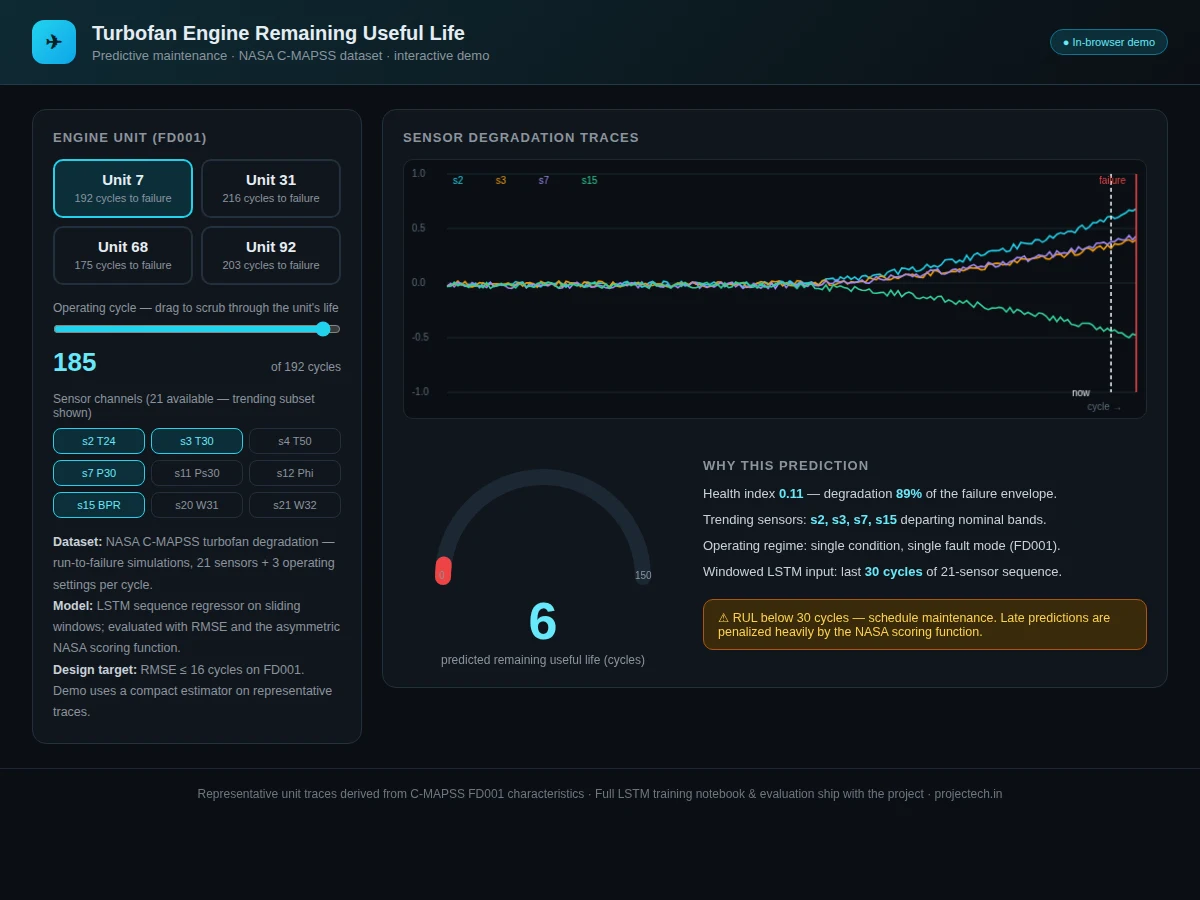
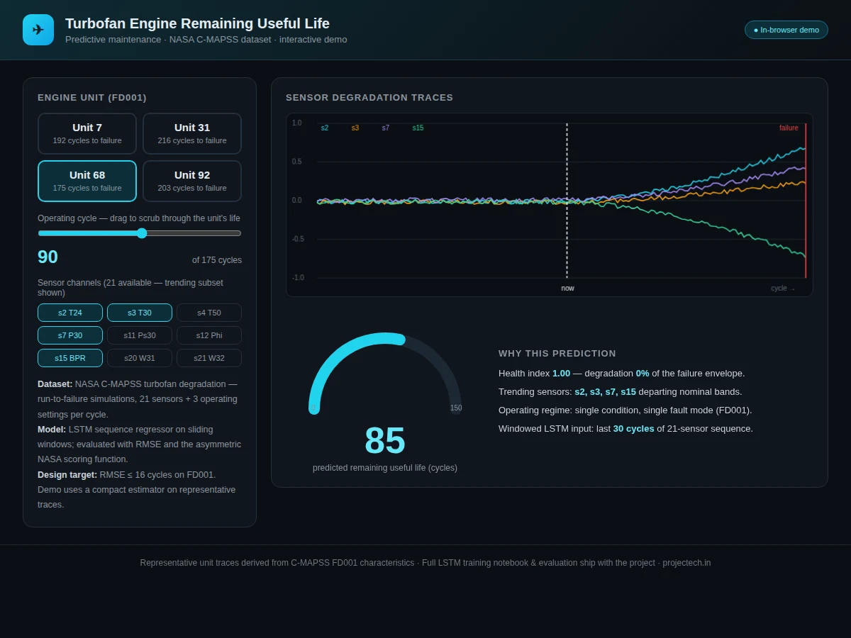
- In the demo, scrubbing the cycle slider feeds the corresponding window through the saved model and renders the RUL estimate, health index and sensor traces.
Tech stack:
- Python 3, TensorFlow/Keras (LSTM)
- NumPy, Pandas (sequence handling)
- Matplotlib (degradation plots)
- scikit-learn (metrics, scaling)
- Jupyter Notebook (training & evaluation)
- HTML5 canvas + JavaScript (interactive demo)
- NASA C-MAPSS dataset
Dataset & model details
- Dataset: NASA C-MAPSS (Commercial Modular Aero-Propulsion System Simulation) turbofan degradation dataset, NASA Prognostics Center of Excellence (Saxena & Goebel) — run-to-failure multivariate time series; FD001 subset: 100 training engines, 100 test engines, 21 sensors + 3 operating settings per cycle, single operating condition and fault mode.
- Task: Regression; input = 30-cycle window of 21-sensor sequence, output = remaining useful life in cycles (non-negative scalar).
- Model: Stacked LSTM: LSTM(100, return sequences) → Dropout → LSTM(50) → Dropout → Dense(1); MSE loss, Adam optimizer; piecewise-linear RUL labels capped at 130 cycles.
- Metrics: RMSE ≤ 16 cycles on FD001 (design target for the built-to-order training run); NASA asymmetric scoring function reported alongside. Published LSTM baselines report RMSE around 12–16 on FD001 in the literature; no figure is claimed as measured until the training run is executed for the order.
| Parameter | Value |
|---|---|
| Input | 30-cycle window × 21 sensors (+ 3 settings) |
| Output | Remaining useful life, cycles (≥ 0) |
| Training engines | 100 (FD001 train split) |
| Test RMSE | ≤ 16 cycles (design target, not a measured claim) |
| Training time | Approximately 30–60 min on a laptop GPU/CPU (expected) |
| Inference | Approximately 5 ms per window on CPU (expected) |
| Model file | Approximately 2–4 MB (.h5, expected) |
| Demo | Single-file web app, runs offline after download |
Project features
- [LSTM RUL regressor] A stacked LSTM reading 30-cycle windows of 21-sensor sequences, outputting remaining cycles as a continuous value.
- [Interactive engine-life demo] Scrub through a sample engine's operating history, watch sensor traces degrade, and see the predicted RUL and health index update live.
- [NASA scoring function] The asymmetric penalty (exponential cost on late predictions) implemented and reported alongside RMSE, as the domain requires.
- [Full training notebook] Data loading, sequence windowing, normalization per operating regime, model definition, training and evaluation in one reproducible notebook.
- [Sensor-trend analysis] Which sensors actually carry degradation signal (and which are flat noise) is analyzed and documented for the report.
- [Piecewise RUL labeling] The standard capped-RUL labeling strategy (constant early life, linear degradation after the knee point) implemented and explained.
- [Exported trained model] Saved weights plus the windowing/preprocessing pipeline so the demo estimates RUL without retraining.
What is included
- Complete training & evaluation Jupyter notebook
- Trained LSTM model file (.h5) with windowing/preprocessing code
- Interactive engine-life demo wired to the trained model
- RMSE + NASA-score evaluation tables and degradation plots
- Project report PDF (background, LSTM theory, labeling rationale, methodology, results)
- PPT presentation for final review
- Viva Q&A preparation document (LSTMs, vanishing gradients, RUL labeling, asymmetric scoring)
Limitations & prerequisites
- C-MAPSS is simulated data — clean compared to real engine telemetry with sensor faults and missing samples; the report states this plainly.
- FD001 covers one operating condition and one fault mode; generalizing across regimes (FD002–FD004) is listed as future scope.
- RMSE ≤ 16 is a design target for the training run, stated honestly — the report documents the actual achieved figure after training.
- The demo's in-browser estimator is a compact illustration of the pipeline; the full trained LSTM ships separately in the deliverables.
- RUL prediction supports maintenance decisions; it does not certify airworthiness — no safety claim is made.
Frequently Asked Questions
Which dataset is used and why?
NASA C-MAPSS — the standard public benchmark for remaining-useful-life prediction, with run-to-failure sensor histories for turbofan engines. Every published method reports on it, so results are directly comparable.
Why an LSTM and not a plain regressor?
Degradation is a temporal process: the story is in how sensors drift over dozens of cycles, not in any single snapshot. LSTMs keep that history in memory; a per-cycle regressor throws it away.
What is the NASA scoring function?
An asymmetric penalty that grows exponentially with error — and punishes late predictions (overestimating remaining life) far more than early ones, because a late prediction can mean an in-service failure.
How does the demo work?
Pick a sample engine and drag the cycle slider: the app feeds the 30-cycle window ending at that cycle through the model and shows predicted RUL, health index and the degrading sensor traces.
Which sensors matter most?
A subset (temperatures, pressures, fan speeds such as sensors 2, 3, 4, 7, 11, 12, 15, 20, 21) trends with degradation; the rest are flat or pure noise. The notebook analyzes and documents this.
Is this project suitable for a final-year project?
Yes — for AI & Machine Learning, Mechanical and Electrical programs. It combines sequence deep learning, a real NASA benchmark, domain-correct evaluation and a working predictive-maintenance demo. Suitable for B.E./B.Tech final-year projects in AI & Machine Learning, Mechanical and Electrical engineering.
Components & software requirements
- Python 3, TensorFlow/Keras (LSTM)
- NumPy, Pandas (sequence handling)
- Matplotlib (degradation plots)
- scikit-learn (metrics, scaling)
- Jupyter Notebook (training & evaluation)
- HTML5 canvas + JavaScript (interactive demo)
- NASA C-MAPSS dataset
Dataset & model details
- Dataset: NASA C-MAPSS (Commercial Modular Aero-Propulsion System Simulation) turbofan degradation dataset, NASA Prognostics Center of Excellence (Saxena & Goebel) — run-to-failure multivariate time series; FD001 subset: 100 training engines, 100 test engines, 21 sensors + 3 operating settings per cycle, single operating condition and fault mode.
- Task: Regression; input = 30-cycle window of 21-sensor sequence, output = remaining useful life in cycles (non-negative scalar).
- Model: Stacked LSTM: LSTM(100, return sequences) → Dropout → LSTM(50) → Dropout → Dense(1); MSE loss, Adam optimizer; piecewise-linear RUL labels capped at 130 cycles.
- Metrics: RMSE ≤ 16 cycles on FD001 (design target for the built-to-order training run); NASA asymmetric scoring function reported alongside. Published LSTM baselines report RMSE around 12–16 on FD001 in the literature; no figure is claimed as measured until the training run is executed for the order.
Delivery information
Built-to-order project. Delivery timeline is shared after order confirmation based on current queue.
Support terms
Complete documentation, setup guide, and viva preparation included. Support for setup and explanation provided.