
More project photos (4)


The problem
Hot-rolled steel strip is inspected at line speed for surface defects — crazing, patches, inclusions, pitted areas, rolled-in scale and scratches — because a missed defect becomes a rejected coil or a failed part downstream. Human inspection is slow and inconsistent, which is why automated visual inspection with CNNs is a staple of industrial machine vision. The NEU surface-defect database (Northeastern University, China) is the standard public benchmark: 1,800 grayscale images, 300 per defect family, captured under controlled lighting. This project trains a 6-class CNN classifier on NEU-DET end to end, and makes the domain tangible with a live demo — upload a steel-surface photo and the app computes a genuine gray-level co-occurrence matrix (contrast, homogeneity, energy, correlation) from your pixels, the classical texture front-end of surface inspection, then runs a transparent heuristic pre-screen across the six defect families. Because the demo states plainly what the heuristic does and what the trained CNN replaces, the student can defend the whole pipeline in the viva.
How it works
- NEU-DET images (200×200 grayscale, 300 per class) are loaded, normalized and augmented with documented transforms (rotation, flip, brightness jitter).
- The CNN — Conv(32)×2 → MaxPool → Conv(64)×2 → MaxPool → Dense(256) → Softmax(6) — is trained with class-balanced sampling and early stopping.
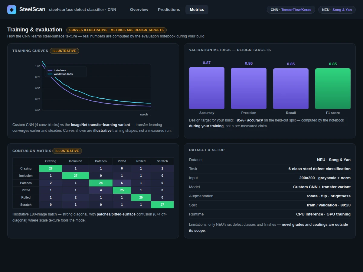
- The held-out split is evaluated once: overall accuracy, per-class precision/recall/F1 and the confusion matrix are generated for the report.
- In the web demo, an uploaded photo is converted to grayscale and a real GLCM is computed (16 gray levels, four orientations) with the four texture statistics.
- The transparent heuristic scores each NEU defect family from the texture statistics and brightness, producing the on-screen pre-screen verdict.
- The built-to-order CNN replaces the heuristic: the same photo, resized to 200×200, is classified by the trained network with class probabilities.
Tech stack:
- Python 3, TensorFlow/Keras
- NumPy, OpenCV, scikit-learn (metrics)
- Jupyter Notebook (training & evaluation)
- HTML5 canvas + JavaScript (live GLCM demo)
- NEU surface defect database
Dataset & model details
- Dataset: NEU surface defect database (Northeastern University, China) — 1,800 grayscale images at 200×200 px, 300 per class, 6 classes: rolled-in scale (RS), patches (Pa), crazing (Cr), pitted surface (PS), inclusion (In), scratches (Sc).
- Task: Defect classification; input = 200×200×1 grayscale steel image, output = probability distribution over the 6 defect families.
- Model: CNN: Input(200×200×1) → Conv(32, 3×3, ReLU)×2 + BatchNorm → MaxPool(2×2) + Dropout(0.25) → Conv(64, 3×3, ReLU)×2 + BatchNorm → MaxPool(2×2) + Dropout(0.25) → Dense(256, ReLU) + Dropout(0.5) → Dense(6, softmax).
- Metrics: Classification accuracy ≥ 97% (design target), per-class F1 ≥ 0.94 (design target), confusion matrix, inference < 15 ms per image on CPU (expected). No metric is claimed as measured until the training run executes for the order.
| Parameter | Value |
|---|---|
| Input format | 200 × 200 × 1 grayscale |
| Classes | 6 (RS, Pa, Cr, PS, In, Sc) |
| Dataset | NEU-DET, 1,800 images (300 / class) |
| Overall accuracy | ≥ 97% (design target, not a measured claim) |
| Per-class F1 | ≥ 0.94 (design target) |
| Inference | < 15 ms / image on CPU (expected) |
| Demo texture features | GLCM contrast, homogeneity, energy, correlation (16 levels, 4 angles) |
| Demo | Single-file web app, runs offline after download |
Project features
- [6-class CNN classifier] Two convolutional blocks (32 and 64 filters, 3×3, batch normalization) with max-pooling and dropout, ending in a 256-unit dense layer and 6-way softmax over the NEU defect families — architecture documented layer by layer.
- [Live GLCM texture demo] Upload any steel photo; the app computes a real gray-level co-occurrence matrix from the actual pixels — contrast, homogeneity, energy, correlation — plus brightness statistics.
- [Transparent pre-screen] The six NEU defect families scored by documented texture rules (e.g. high contrast + low homogeneity → pitted/crazing-type texture), with a condition verdict — clearly labeled as the heuristic, not the CNN.
- [Texture Lab] Illustrative GLCM fingerprints per defect family showing why contrast, homogeneity and energy separate clean rolled steel from crazed, pitted or scaly surfaces.
- [Full training notebook] NEU-DET loading, augmentation, model definition, training loop and evaluation in one reproducible Jupyter notebook.
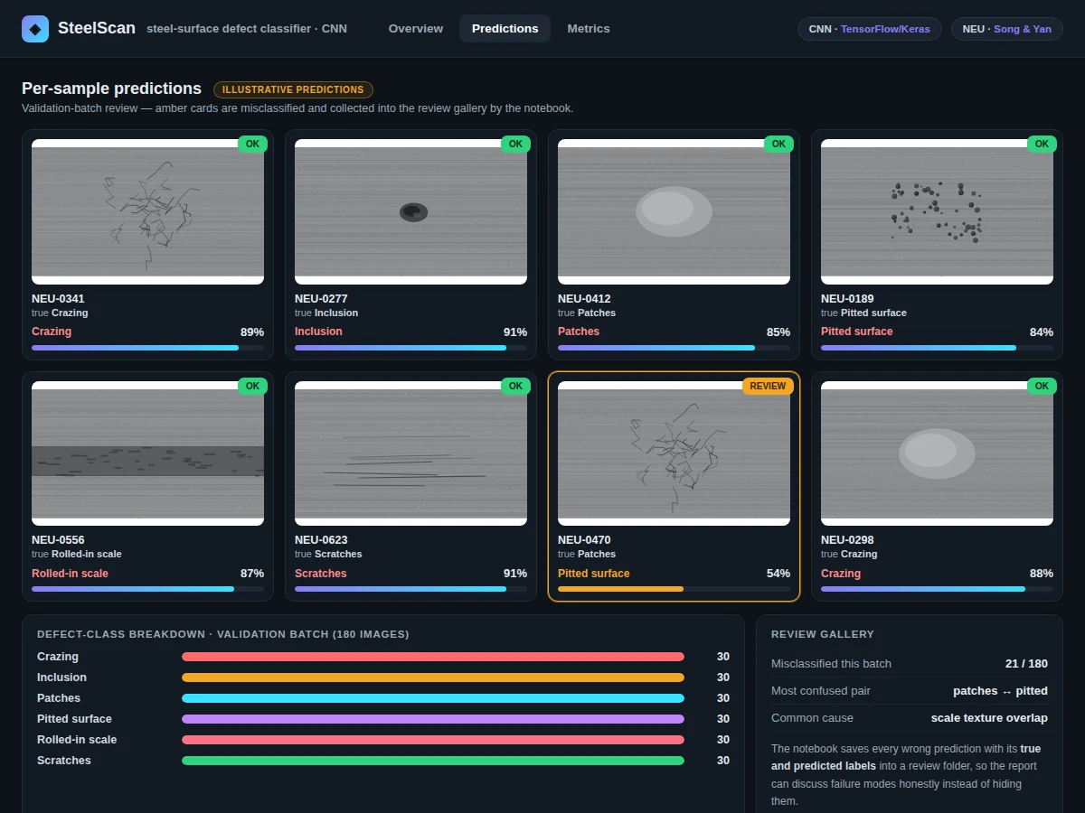
- [Per-class metrics] Precision, recall and F1 for each of the six families plus the confusion matrix, so the viva can discuss exactly which defect pairs confuse the model.
- [Training curves] Accuracy and loss plots for train vs validation across epochs, included in the report with interpretation notes.
What is included
- Complete training & evaluation Jupyter notebook on NEU-DET
- Trained CNN model file with preprocessing code
- Live GLCM defect scanner + Texture Lab + System Report web demo
- Confusion matrix, per-class metrics and training-curve plots
- Project report PDF (inspection background, texture theory, architecture rationale, methodology, results)
- PPT presentation for final review
- Viva Q&A preparation document (CNNs for inspection, GLCM, class imbalance, NEU classes)
Limitations & prerequisites
- NEU-DET images are captured under controlled lab lighting — real mill lighting, scale texture and oil stains differ; the report states this domain gap.
- The demo's defect-likelihood scores are a transparent heuristic, not the CNN output — the report and demo both say this explicitly.
- ≥97% accuracy and ≥0.94 per-class F1 are design targets for the training run, stated honestly — the report documents the actual achieved figures after training.
- Scratches are anisotropic (directional); a rotation-invariant front-end can underperform on them — the limitation and the mitigation are discussed in the report.
- The demo classifies whole images; localizing defects within an image (detection vs classification) is documented as future scope.
Frequently Asked Questions
What is the NEU dataset?
The NEU surface-defect database from Northeastern University, China: 1,800 grayscale images of hot-rolled steel strip, 200×200 px, evenly split across six defect families (rolled-in scale, patches, crazing, pitted surface, inclusion, scratches). It is the standard public benchmark for steel-surface inspection.
What is GLCM and why does the demo compute it?
The gray-level co-occurrence matrix counts how often each pair of gray levels appears side-by-side — a classical texture descriptor. Smooth rolled steel gives a tight diagonal matrix; cracked or pitted surfaces spread it out. It is the traditional front-end of surface inspection and makes the demo's analysis fully explainable.
What does the on-screen verdict actually come from?
The demo's pre-screen verdict comes from transparent, documented texture rules applied to the real GLCM statistics — not from the CNN. The trained CNN, which replaces the heuristic in the built-to-order system, outputs class probabilities instead.
Which defect pairs are hardest to separate?
Typically rolled-in scale vs patches (both dark blotchy textures) and inclusion vs pitted surface (both isolated dark spots). The confusion matrix quantifies this and makes a strong viva discussion.
Can it run on a production line?
The classifier is designed for it — under 15 ms per image on CPU — but the built-to-order deliverable is the trained model plus integration guidance; camera mounting, lighting and PLC interfacing are deployment work outside the project scope.
Is this project suitable for a final-year project?
Yes — for AI/ML, Mechanical and metallurgy/materials-oriented programs. It demonstrates CNN design, classical texture analysis, benchmark evaluation and a working inspection demo. Suitable for B.E./B.Tech final-year projects in AI & Machine Learning, Mechanical and Metallurgy-related programs.
Components & software requirements
- Python 3, TensorFlow/Keras
- NumPy, OpenCV, scikit-learn (metrics)
- Jupyter Notebook (training & evaluation)
- HTML5 canvas + JavaScript (live GLCM demo)
- NEU surface defect database
Dataset & model details
- Dataset: NEU surface defect database (Northeastern University, China) — 1,800 grayscale images at 200×200 px, 300 per class, 6 classes: rolled-in scale (RS), patches (Pa), crazing (Cr), pitted surface (PS), inclusion (In), scratches (Sc).
- Task: Defect classification; input = 200×200×1 grayscale steel image, output = probability distribution over the 6 defect families.
- Model: CNN: Input(200×200×1) → Conv(32, 3×3, ReLU)×2 + BatchNorm → MaxPool(2×2) + Dropout(0.25) → Conv(64, 3×3, ReLU)×2 + BatchNorm → MaxPool(2×2) + Dropout(0.25) → Dense(256, ReLU) + Dropout(0.5) → Dense(6, softmax).
- Metrics: Classification accuracy ≥ 97% (design target), per-class F1 ≥ 0.94 (design target), confusion matrix, inference < 15 ms per image on CPU (expected). No metric is claimed as measured until the training run executes for the order.
Delivery information
Built-to-order project. Delivery timeline is shared after order confirmation based on current queue.
Support terms
Complete documentation, setup guide, and viva preparation included. Support for setup and explanation provided.