
More project photos (2)
The problem
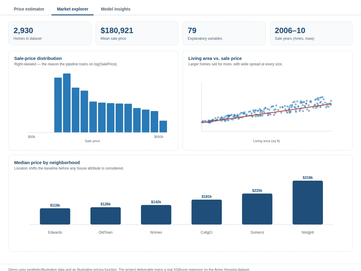
A home is the largest purchase most families ever make, yet its price is still usually set by slow, expensive and partly subjective appraisals — while the online estimators buyers actually use are black boxes that never explain a number. The underlying problem is a regression over messy, mixed data: dozens of attributes (living area, overall quality, garage capacity, basement finish, neighborhood, year built) interact non-linearly, some values are missing, and sale prices are heavily right-skewed. This project applies it to the Ames Housing dataset (2,930 homes, 79 explanatory variables, a standard regression benchmark): missing-value handling per feature type, ordinal encoding of quality ratings, a log transform of the skewed SalePrice target, XGBoost training with early stopping and cross-validation, holdout evaluation with RMSE, MAE and R-squared, SHAP-based feature analysis, and a demo that estimates any home's price from sliders and prices the effect of renovations.
How it works
- The Ames Housing dataset (2,930 homes, 79 explanatory variables) is loaded; missing values are imputed per feature type, quality ratings ordinal-encoded, and SalePrice log-transformed to tame its right skew.
- The data is split into train and holdout sets (e.g. 80/20); the target used for training is log(SalePrice), converted back to dollars at inference.
- An XGBoost regressor is trained with early stopping on a validation fold; hyperparameters (max depth, learning rate, regularization) are tuned with cross-validation.
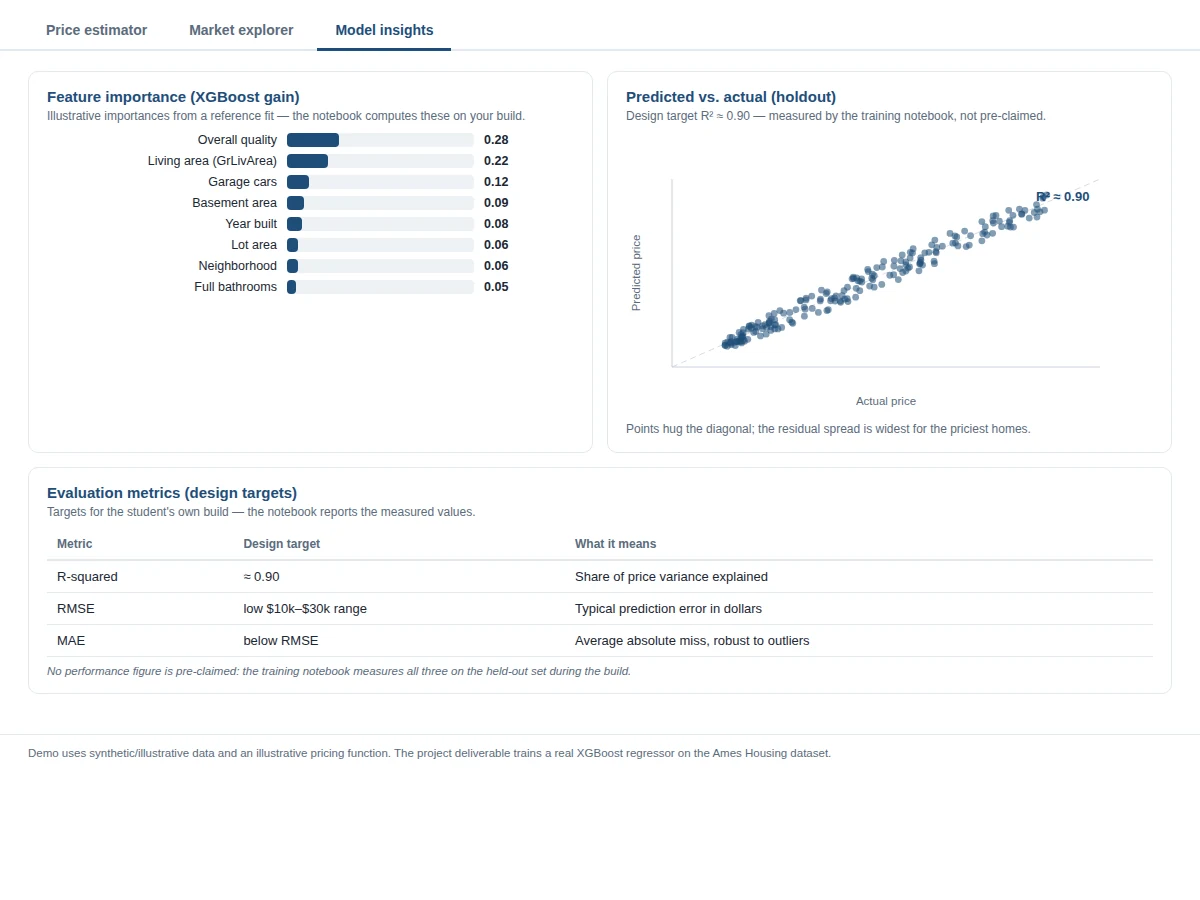
- The holdout set is evaluated with RMSE, MAE and R-squared, plus predicted-vs-actual and residual plots that reveal where the model under- or over-predicts.
- SHAP values and gain importance identify the strongest price drivers — overall quality, living area, garage capacity — for the report's analysis section.
- At inference, the demo encodes a home's attributes with the same pipeline, predicts log-price, exponentiates it, and breaks the estimate down by feature contribution.
Tech stack:
- Python 3.10, XGBoost (gradient-boosted regression, early stopping)
- scikit-learn (pipelines, cross-validation, metrics)
- pandas, NumPy (data wrangling and feature tables)
- Matplotlib, Seaborn (predicted-vs-actual, residuals, importance plots)
- SHAP (feature contribution explanations)
- Jupyter notebook (buyer-run training and evaluation)
- Streamlit demo app (price estimator, renovation simulator, dashboards)
| Parameter | Value |
|---|---|
| Model | XGBoost regressor (gradient-boosted trees, early stopping, cross-validation) |
| Dataset | Ames Housing — 2,930 homes, 79 explanatory variables (De Cock, 2011) |
| Task | Regression on SalePrice (log-transformed for training) |
| Preprocessing | Per-type missing-value imputation, ordinal encoding of quality ratings, log target transform |
| Evaluation | RMSE, MAE, R-squared, predicted-vs-actual and residual plots — computed on your holdout by the notebook |
| Design target | R-squared approximately 0.90 with RMSE in the low tens of thousands of dollars; a development target, not a guaranteed result |
| Output | Predicted sale price in USD with per-feature contribution breakdown |
| Inference | Interactive slider estimator in the demo app plus batch CSV scoring |
Project features
- [Ames Housing data pipeline] Loads the Ames dataset (2,930 homes, 79 features), imputes missing values per feature type, ordinal-encodes quality ratings (Excellent to Poor), and log-transforms the skewed SalePrice target.
- [XGBoost regressor with early stopping] Trains gradient-boosted trees with early stopping on a validation fold and cross-validation, with max depth, learning rate and regularization exposed as tunable hyperparameters.
- [SHAP and gain-based importance] Ranks price drivers — overall quality, living area and garage capacity typically top the list — with gain importance bars and SHAP summary plots the report can analyze.
- [Interactive price estimator] Move sliders for overall quality, living area, garage cars, basement area, year built and lot area and get an instant price estimate with a per-feature contribution breakdown.
- [Renovation simulator] Upgrade the kitchen or overall quality rating in the demo and see the predicted price delta — a concrete "what is the upgrade worth" analysis for the report.
- [Evaluation dashboard] Predicted-vs-actual scatter, residual plots, RMSE, MAE and R-squared on the held-out set, all computed by the notebook during the build.
- [Neighborhood price explorer] Median sale prices and price distributions across Ames neighborhoods, showing how location shifts the baseline.
- [Comparable-homes finder] Finds the nearest neighbors of an input home in feature space and shows their actual sale prices beside the prediction.
What is included
- Complete source code (data pipeline, training, evaluation, demo app)
- Jupyter training and evaluation notebook (buyer-run procedure on the Ames dataset)
- Project report PDF (background, methodology, SHAP analysis, evaluation, error analysis)
- PPT presentation for final review
- Viva Q&A preparation document (gradient boosting, log transform, RMSE vs MAE, SHAP, overfitting control)
- Setup guide (environment, dataset download, running the notebook and demo)
Limitations & prerequisites
- The Ames data covers one Iowa city from 2006–2010; it does not represent current prices, other cities, or today's interest-rate environment — this is a teaching benchmark, not a valuation service.
- The model interpolates within the training distribution; unusual luxury homes or extreme feature values extrapolate poorly, as the residual plots show.
- Macroeconomic drivers (interest rates, local employment, school ratings beyond the dataset) are outside the feature set.
- The renovation simulator estimates price effects of upgrades, not their construction cost — return-on-investment needs cost data the project does not include.
- Currency and units are US dollars and square feet throughout, matching the dataset.
Frequently Asked Questions
Which dataset is used?
The Ames Housing dataset (2,930 residential sales, 79 explanatory variables, compiled by De Cock for a statistics-education paper and hosted on Kaggle). It covers living area, overall quality, garage, basement, lot, neighborhood, year built and the SalePrice target.
Why XGBoost instead of linear regression?
House prices depend on non-linear interactions (quality times living area, diminishing returns on lot size) that linear models miss, and the data has mixed types with missing values. XGBoost handles all of this natively and consistently tops this benchmark among tabular models.
Is the accuracy guaranteed?
No. The design target is R-squared near 0.90 with RMSE in the low tens of thousands of dollars on the holdout — realistic for XGBoost on Ames — but the notebook measures the actual values on your build, and the report documents those numbers, not a promise.
Why is the sale price log-transformed?
SalePrice is heavily right-skewed (a few very expensive homes). Training on log(SalePrice) makes the error distribution symmetric so the model is not dominated by the priciest homes; predictions are converted back to dollars with the exponential at inference.
Can it be retrained on another city's data?
Yes. Any tabular listing dataset with a price column works: adjust the encoding step to the new columns and retrain in the notebook. The demo's estimator sliders can be re-mapped to the new feature set.
What will the project report analyze?
SHAP and gain-based feature rankings, the predicted-vs-actual and residual plots (where the model systematically errs), the renovation simulator's upgrade scenarios, and the neighborhood price comparison.
Suitable for B.E./B.Tech final-year projects in Computer Science, AI/ML and Data Science.
Components & software requirements
- Python 3.10, XGBoost (gradient-boosted regression, early stopping)
- scikit-learn (pipelines, cross-validation, metrics)
- pandas, NumPy (data wrangling and feature tables)
- Matplotlib, Seaborn (predicted-vs-actual, residuals, importance plots)
- SHAP (feature contribution explanations)
- Jupyter notebook (buyer-run training and evaluation)
- Streamlit demo app (price estimator, renovation simulator, dashboards)
Delivery information
Built-to-order project. Delivery timeline is shared after order confirmation based on current queue.
Support terms
Complete documentation, setup guide, and viva preparation included. Support for setup and explanation provided.