
More project photos (2)
The problem
Telling a rose from a camellia is easy; telling 102 flower species apart — many differing only in petal texture or stamen shape — is a genuinely hard vision problem called fine-grained classification. The Oxford 102 Flowers dataset (8,189 photographs, 102 categories, some with as few as 40 images) is the classic benchmark for it, and it is deliberately awkward: too small to train a deep network from scratch, too fine-grained for a shallow one. The right answer is transfer learning, and this project does it the rigorous way — first a linear probe on a frozen ResNet-50 backbone, then fine-tuning of the top residual blocks with a low learning rate and discriminative scheduling. A web demo makes the result tangible: pick a bloom photo and see the ranked top-5 species with confidence scores, exactly like a plant-identification app.
How it works
- The Oxford 102 Flowers dataset (8,189 images, 102 classes, 40–258 images per class) is loaded with the official train/validation/test splits; train+validation are combined for fitting.
- Images are resized to 224×224×3 and normalized with ImageNet statistics; augmentation applies random crops, horizontal flips and color jitter.
- Phase 1 (linear probe): the ResNet-50 backbone stays frozen while only the new classification head trains, establishing a baseline.
- Phase 2 (fine-tuning): the top residual blocks are unfrozen and trained with a 10× lower learning rate plus early stopping on validation loss.
- The held-out test set is evaluated once: top-1/top-5 accuracy, macro F1 and a confusion analysis over the most-mixed species pairs.
- In the web demo, a bloom photo passes through identical preprocessing and the saved model, and the app renders the ranked top-5 species with confidence bars.
Tech stack:
- Python 3, PyTorch (torchvision ResNet-50)
- Transfer learning (ImageNet weights)
- NumPy, PIL (preprocessing)
- Matplotlib, scikit-learn (evaluation)
- Jupyter Notebook (training)
- HTML/CSS/JavaScript (web demo)
- Oxford 102 Flowers dataset (VGG, Oxford)
Dataset & model details
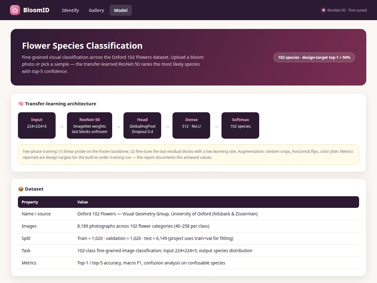
- Dataset: Oxford 102 Flowers — Visual Geometry Group, University of Oxford (Nilsback & Zisserman). 8,189 photographs across 102 flower categories (40–258 images per class); official split ≈ 1,020 train / 1,020 validation / 6,149 test.
- Task: 102-class fine-grained image classification; input = 224×224×3 image, output = probability distribution over 102 species.
- Model: ResNet-50 (ImageNet pretrained) → GlobalAveragePooling → Dropout(0.4) → Dense(512, ReLU) → Dense(102, softmax); two-phase training: frozen-backbone linear probe, then fine-tune top blocks at low LR.
- Metrics: Top-1 accuracy (design target ≈ 94%), top-5 accuracy (design target ≈ 99%), macro F1, confusable-species analysis. No accuracy is claimed as measured until the training run is executed for the order.
| Parameter | Value |
|---|---|
| Input format | 224 × 224 × 3 RGB, ImageNet-normalized |
| Classes | 102 flower species |
| Model parameters | Approximately 24M (ResNet-50 + head) |
| Top-1 accuracy | ≈ 94% (design target, not a measured claim) |
| Top-5 accuracy | ≈ 99% (design target) |
| Training time | Approximately 1–2 hrs on a free Colab GPU (expected) |
| Inference | Approximately 60 ms per image on CPU (expected) |
| Model file | Approximately 95 MB (.pth, expected) |
| Demo | Single-file web app, runs offline after download |
Project features
- [102-species classifier] ResNet-50 fine-tuned on Oxford 102 Flowers — identifies species from a single bloom photograph with top-5 ranking.
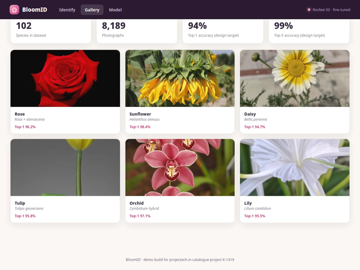
- [Live web demo] Select sample blooms (rose, sunflower, daisy, tulip, orchid, lily) and get the predicted species, Latin name and top-5 confidence bars.
- [Two-phase transfer learning] Documented linear-probe-then-fine-tune schedule with layer-wise learning rates, exactly as the literature recommends.
- [Full training notebook] Dataset loading, 224×224 preprocessing, augmentation (crops, flips, color jitter), training loops and evaluation in one reproducible notebook.
- [Top-1 / top-5 evaluation] Accuracy plus macro F1 and a confusable-species analysis (which species the model mixes up, and why).
- [Training curves & error gallery] Validation curves and a misclassified-samples gallery with interpretation notes for the report.
- [Exported fine-tuned model] Saved weights plus preprocessing code, so the demo runs the real network without retraining.
What is included
- Complete training & evaluation Jupyter notebook (PyTorch)
- Fine-tuned ResNet-50 weights with preprocessing code
- Web demo wired to the trained model (sample blooms + top-5 ranking)
- Training curves, error gallery and confusable-species analysis
- Project report PDF (background, transfer-learning theory, methodology, results)
- PPT presentation for final review
- Viva Q&A preparation document (fine-grained classification, fine-tuning, top-k metrics)
Limitations & prerequisites
- 102 species from one dataset — garden varieties outside these classes will be force-fit to the nearest species.
- ≈ 94% top-1 / 99% top-5 are design targets for the training run, stated honestly — the report documents the actual achieved figures after training.
- Classes with only ~40 training images remain the weakest; the report quantifies this per-class.
- The model expects a reasonably centered bloom photo; wide garden scenes with tiny flowers are out of scope.
- This is a teaching build, not a botanical reference — no claim is made about taxonomic authority.
Frequently Asked Questions
Which dataset is used and why?
Oxford 102 Flowers from the Visual Geometry Group, University of Oxford — 8,189 photos across 102 species. It is the standard fine-grained classification benchmark: small enough to need transfer learning, hard enough to prove it works.
What is the two-phase training?
Phase 1 trains only the new classification head on a frozen backbone (fast, stable baseline). Phase 2 unfreezes the top residual blocks and continues at a much lower learning rate so pretrained features adapt without being destroyed.
How does the web demo work?
Pick a sample bloom; the app applies the exact training preprocessing and the saved model returns the top-5 species with confidence bars, plus the Latin name of the top prediction.
Which species confuse the model most?
Visually similar pairs — e.g. daisy vs coneflower, tulip vs lily. The report's confusable-species analysis shows the worst pairs with example images, which makes a strong viva discussion.
Why PyTorch instead of Keras?
Either works; this build uses PyTorch with torchvision's pretrained ResNet-50 because its fine-tuning workflow (parameter groups, LR scheduling) is explicit and easy to explain in a viva.
Is this project suitable for a final-year project?
Yes — for Computer Science, IT and AI/ML programs. It demonstrates transfer learning done properly, fine-grained evaluation and a working deployment demo. Suitable for B.E./B.Tech final-year projects in Computer Science, IT and AI & Machine Learning.
Components & software requirements
- Python 3, PyTorch (torchvision ResNet-50)
- Transfer learning (ImageNet weights)
- NumPy, PIL (preprocessing)
- Matplotlib, scikit-learn (evaluation)
- Jupyter Notebook (training)
- HTML/CSS/JavaScript (web demo)
- Oxford 102 Flowers dataset (VGG, Oxford)
Dataset & model details
- Dataset: Oxford 102 Flowers — Visual Geometry Group, University of Oxford (Nilsback & Zisserman). 8,189 photographs across 102 flower categories (40–258 images per class); official split ≈ 1,020 train / 1,020 validation / 6,149 test.
- Task: 102-class fine-grained image classification; input = 224×224×3 image, output = probability distribution over 102 species.
- Model: ResNet-50 (ImageNet pretrained) → GlobalAveragePooling → Dropout(0.4) → Dense(512, ReLU) → Dense(102, softmax); two-phase training: frozen-backbone linear probe, then fine-tune top blocks at low LR.
- Metrics: Top-1 accuracy (design target ≈ 94%), top-5 accuracy (design target ≈ 99%), macro F1, confusable-species analysis. No accuracy is claimed as measured until the training run is executed for the order.
Delivery information
Built-to-order project. Delivery timeline is shared after order confirmation based on current queue.
Support terms
Complete documentation, setup guide, and viva preparation included. Support for setup and explanation provided.