
More project photos (3)


The problem
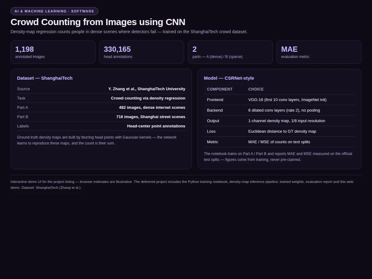
Counting people in dense crowds defeats bounding-box detectors: heads merge, overlap and shrink with perspective until boxes are meaningless. Density-map regression sidesteps detection entirely — the network predicts a per-pixel density whose spatial sum is the head count. The ShanghaiTech dataset (Zhang et al.) provides 1,198 images with 330,165 head-center annotations across dense internet scenes (Part A) and Shanghai street scenes (Part B): the standard benchmark. CSRNet showed that dilated convolutions give counting the large receptive fields it needs without pooling away resolution. This project trains that architecture, evaluates MAE/MSE on the official test splits, and demos heatmap overlays with overcrowding alerts for venue-safety use.
Uploads a crowd scene photo in the demo UI.
Follow the working sequence
How it works
- Head-center annotations are blurred with Gaussian kernels to create ground-truth density maps.
- A VGG-16 frontend (first 10 conv layers, ImageNet-initialized) extracts features.
- Six dilated convolution layers (rate 2) expand the receptive field without downsampling.
- The network outputs a single-channel density map at 1/8 input resolution, trained with Euclidean loss.
- Summing the map gives the head count; thresholding it into bands gives zone alerts.
- Training runs on ShanghaiTech Parts A and B; evaluation reports MAE/MSE per official split.
Tech stack:
- Python 3.10, PyTorch
- CSRNet-style fully-convolutional network
- ShanghaiTech dataset (Zhang et al.)
- OpenCV, NumPy (density maps, overlays)
- Flask (demo backend)
- HTML/CSS/JavaScript (demo UI)
- Git
Dataset & Model Details
- Dataset: ShanghaiTech — 1,198 images, 330,165 head-center annotations; Part A: 482 dense internet scenes; Part B: 716 Shanghai street scenes; source: Y. Zhang et al., ShanghaiTech University.
- Model input: crowd scene image. Output: single-channel density map; count = spatial sum.
- Architecture: VGG-16 frontend (10 conv layers) → 6 dilated conv layers (rate 2) → density map; Euclidean loss vs. Gaussian-blurred ground truth.
- Metric: MAE / MSE of counts on the official test splits, measured after training. No figure is claimed before the training run.
| Parameter | Value |
|---|---|
| Task | Crowd counting via density regression |
| Input | Crowd scene photo |
| Output | Density map + head count + alert level |
| Alert threshold | Configurable persons/m² (default ~3.0) |
| Inference | Under 1 s per frame on CPU (design target) |
| Demo | Scene upload + heatmap + alerts |
Project features
- [Density-map regression] Fully-convolutional network predicts a per-pixel density map; the count is its spatial sum — no boxes needed.
- [CSRNet-style architecture] VGG-16 frontend plus six dilated convolution layers for large receptive fields without resolution loss.
- [Heatmap overlays] Predicted density rendered green→yellow→red over the scene so crowd concentration is visible.
- [Overcrowding alerts] Zone-level density thresholds raise LOW/MEDIUM/HIGH badges against a configurable persons/m² limit.
- [Gaussian ground truth] Head annotations blurred with geometry-adaptive kernels to build training density maps.
- [Honest split evaluation] MAE/MSE measured separately on Part A (dense) and Part B (street) test splits.
- [Scene demo] Upload a crowd photo; get the heatmap, count and alert status.
What is included
- Python training notebook (density-map training, Gaussian GT generation, evaluation)
- Density-map inference pipeline + heatmap visualization code
- Trained model weights
- Test-split evaluation: MAE/MSE on Parts A and B from the actual run
- Web demo (scene upload, heatmap overlay, count, alert badges)
- Project report PDF (methodology, split comparison, measured results)
- PPT presentation for final review
- Viva Q&A preparation document
Limitations & prerequisites
- Estimates, not exact counts — dense scenes carry higher error, and the Part A vs B numbers show it.
- Extreme perspective distortion and night scenes degrade accuracy without domain-specific retraining.
- Persons/m² figures are estimates from the density map, not calibrated measurements.
- The model counts visible heads; fully occluded people are missed like any vision system.
- GPU recommended for training; inference runs on CPU.
Frequently Asked Questions
Why not just use YOLO to detect people?
In dense crowds heads merge and overlap, so detectors undercount badly. Density regression skips boxes entirely and stays accurate exactly where detectors collapse — the Part A evaluation demonstrates this.
What is a density map?
A per-pixel map where brightness means people-per-pixel. It is built by blurring head-center annotations with Gaussian kernels; the network learns to reproduce it, and its sum is the count.
What dataset is used?
ShanghaiTech: 1,198 images with 330,165 head annotations, split into dense Part A and street-scene Part B — the standard crowd-counting benchmark.
How are overcrowding alerts decided?
The density map is thresholded into low/medium/high bands; zones above the configured persons/m² limit raise the alert badge for venue staff.
How accurate is it?
The notebook measures MAE and MSE on the official test splits and reports them separately for dense vs street scenes — no pre-claimed numbers.
Is this project suitable for a final-year project?
Yes — for Computer Science, IT and AI/ML programs. It teaches regression-style computer vision, a genuinely different paradigm from detection, with a venue-safety application. Suitable for B.E./B.Tech final-year projects in Computer Science, Information Technology and AI/ML.
Components & software requirements
- Python 3.10, PyTorch
- CSRNet-style fully-convolutional network
- ShanghaiTech dataset (Zhang et al.)
- OpenCV, NumPy (density maps, overlays)
- Flask (demo backend)
- HTML/CSS/JavaScript (demo UI)
- Git
Dataset & Model Details
- Dataset: ShanghaiTech — 1,198 images, 330,165 head-center annotations; Part A: 482 dense internet scenes; Part B: 716 Shanghai street scenes; source: Y. Zhang et al., ShanghaiTech University.
- Model input: crowd scene image. Output: single-channel density map; count = spatial sum.
- Architecture: VGG-16 frontend (10 conv layers) → 6 dilated conv layers (rate 2) → density map; Euclidean loss vs. Gaussian-blurred ground truth.
- Metric: MAE / MSE of counts on the official test splits, measured after training. No figure is claimed before the training run.
Delivery information
Built-to-order project. Delivery timeline is shared after order confirmation based on current queue.
Support terms
Complete documentation, setup guide, and viva preparation included. Support for setup and explanation provided.
Download free synopsis (PDF)
Enter your name and WhatsApp number — the synopsis PDF downloads immediately. We may send occasional project updates on WhatsApp; no spam.