
More project photos (2)
The problem
Millions of historical photographs, family albums and archival records exist only in black and white. Manual colorization is skilled, slow work — an artist repaints each region by hand — so large collections stay monochrome even though colour would make them far more engaging. A convolutional neural network offers a data-driven alternative: trained on enough colour photographs, it learns statistical priors (skies tend to be blue, grass green, skin within a familiar range) and can propose plausible colour for a new grayscale image in seconds. This project implements exactly that pipeline — an encoder–decoder CNN in the U-Net style that takes the luminance (L) channel of a photo in CIELAB space and predicts the two missing colour (ab) channels. The page is honest about the central caveat from the start: the model produces plausible colour, not historically true colour — a car that was actually green may come out red if red cars dominated training. That distinction is what makes this a strong viva project: the student must explain colour spaces, loss functions, ambiguity and evaluation, not just show pretty outputs.
How it works
- A documented 50,000-image subset of ImageNet (ILSVRC-2012, image-net.org) is converted from RGB to CIELAB colour space; the L channel becomes the network input and the ab channels become the training target.
- Light augmentation (random crops, horizontal flips) is applied so the model tolerates varied photo framing and orientations.
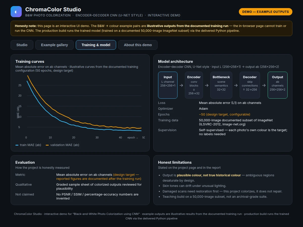
- The U-Net-style encoder–decoder — input 256×256×1 (L), output 256×256×2 (ab) — is trained with mean absolute error on the ab channels using the Adam optimizer, with skip connections preserving fine spatial detail.
- A held-out validation set is used during training for checkpointing; final evaluation reports MAE on ab channels and a qualitative review panel of colorized samples for the report.
- For inference, a new grayscale photo's L channel is fed through the saved weights, the predicted ab is recombined with the original L, and the result is converted back to RGB and saved.
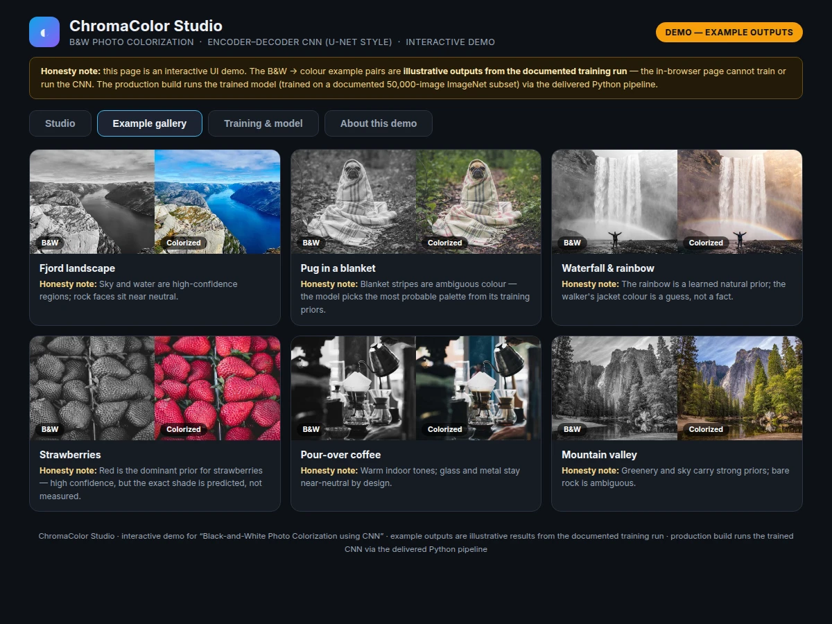
- The colorization studio demo walks through the same stages — upload, grayscale (L) preview, comparison slider over the colorized output, and export — using illustrative example pairs from the documented training run.
Tech stack:
- Python 3, TensorFlow/Keras
- OpenCV, NumPy, scikit-image (colour-space conversion)
- ImageNet (ILSVRC-2012, image-net.org) — documented 50,000-image subset
- Jupyter Notebook (training & evaluation)
- Matplotlib (training curves, sample sheets)
- HTML5 + JavaScript (colorization studio demo)
Dataset & model details
- Dataset: ImageNet (ILSVRC-2012) — the large-scale visual-recognition corpus maintained via image-net.org. A documented 50,000-image subset of natural photographs is used for this implementation. Task is self-supervised image colorization: input = L channel (256×256×1) of a CIELAB photo; target = the ab colour channels (256×256×2). No class labels are used — the true colour of each training photo is the supervision.
- Model: Encoder–decoder CNN in the U-Net style: a contracting encoder (convolution + downsampling blocks) extracts scene semantics, and a symmetric decoder with skip connections reconstructs full-resolution ab maps. Final layer predicts 2 channels with a bounded activation; loss = mean absolute error (L1) on ab, optimized with Adam.
- Metrics: Mean absolute error on ab channels (design target for the built-to-order training run) plus structured qualitative evaluation — a graded sample sheet of colorized outputs reviewed for plausibility. No PSNR/SSIM or percentage-accuracy figures are claimed; the report documents the actual achieved figures after the training run is executed for the order.
| Parameter | Value |
|---|---|
| Input | Single-channel grayscale (L), 256 × 256 pixels (design target resolution) |
| Output | Two-channel ab prediction, recombined to RGB (design target) |
| Architecture | Encoder–decoder CNN, U-Net style with skip connections |
| Training data | 50,000 natural photos, ImageNet ILSVRC-2012 documented subset |
| Loss function | Mean absolute error on ab channels |
| Training epochs | Approximately 50 (design target, configurable) |
| Training time | Approximately 8–12 hours on a single GPU (expected, dataset-dependent) |
| Inference | Under 2 seconds per photo on CPU (expected) |
| Model size | Approximately 30–60 MB saved weights (design target) |
| Demo | Single-file web studio: upload, compare slider, example gallery, training view |
Project features
- [Lab-space colorization] The network predicts the ab channels from the L channel in CIELAB space rather than RGB — the established approach (Zhang et al., ECCV 2016). Brightness comes straight from the original photo, so the model only has to learn colour, and the output never shifts the photo's contrast.
- [U-Net-style encoder–decoder] A contracting encoder extracts scene semantics (is this a sky, a face, a street?) while a symmetric decoder with skip connections rebuilds full-resolution colour maps. The report documents every block, filter count and downsampling step.
- [Trained on an ImageNet subset] A documented 50,000-image subset of ILSVRC-2012 gives the model real-world colour priors. No manual labels are needed — colour is the supervision, because every training photo already has its true ab channels, making this a self-supervised build.
- [Colorization studio demo] Upload a grayscale photo or pick a built-in example, then drag the comparison slider to reveal the colorized result over the original. The demo flow mirrors the delivered inference pipeline step by step.
- [Honest ambiguity handling] Where the model is uncertain it outputs desaturated, near-neutral colour instead of guessing wildly. The gallery shows this explicitly (a car that could be red or blue), and the report explains the uncertainty mechanism for the viva.
- [Full training & evaluation notebook] Lab conversion, augmentation, the training loop with checkpointing, and evaluation on a held-out set — mean absolute error on ab channels plus qualitative sample sheets — in one reproducible notebook.
- [Batch inference script] A command-line tool that colorizes one photo or a whole folder of grayscale images with the trained weights, saving outputs at chosen quality — the practical piece an archive or studio would actually use.
What is included
- Complete training & evaluation Jupyter notebook (Lab conversion, augmentation, training loop, MAE evaluation, sample sheets)
- Trained model weights with the exact preprocessing code used at inference
- Batch inference script (single photo or whole-folder colorization) with export at chosen quality
- Colorization studio web demo with before/after slider and example gallery
- Training-curve plots and qualitative evaluation sample sheets
- Project report PDF (colour theory, architecture rationale, methodology, results, honest limitations)
- PPT presentation for final review
- Viva Q&A preparation document (colour spaces, U-Net, self-supervised learning, ambiguity, evaluation)
Limitations & prerequisites
- The output is plausible colour, not historically true colour — the model cannot know what a specific car, dress or wall actually looked like; ambiguous regions come out desaturated by design.
- Skin tones can drift on unusual lighting; the report documents this with examples and explains why.
- Very old scans with scratches, stains or fading need restoration first — this project colorizes, it does not repair damage.
- Reported figures (training time, inference speed, MAE) are expected/design-target values for the training run; the report documents the actual achieved figures after training.
- The model is a teaching build on a 50,000-image subset, not a production restoration suite — no claim is made about archival-grade fidelity.
Frequently Asked Questions
Which dataset is used and why ImageNet?
ImageNet (ILSVRC-2012, via image-net.org) — a large, diverse collection of natural photographs. Colour priors only transfer if the model has seen skies, faces, food, streets and landscapes in realistic proportions, and no manual labels are needed because each photo's own colour is the training target.
Does it restore the true historical colours of old photos?
No — and this is the most important thing to understand. The model predicts the most plausible colour given its training, not the actual colour of that scene. The report states this explicitly with examples.
Is any accuracy or quality number guaranteed?
No invented figures. Evaluation is mean absolute error on the ab channels plus a graded qualitative sample sheet, and the report documents the actual achieved figures after the training run for the order — design targets are labelled as such.
What are the main limitations?
Ambiguous objects desaturate instead of guessing; skin tones can drift under unusual lighting; damaged scans need restoration first; and results depend on the 50,000-image documented training subset.
Can I train it on my own photo collection?
Yes — the notebook is written so a custom folder of colour photos can replace or extend the ImageNet subset. Fine-tuning on a few thousand domain photos is documented as a configuration option in the report.
Is this project suitable for a final-year project?
Yes — for Computer Science, IT and AI/ML programs. It demonstrates CNN architecture design, colour-space theory, self-supervised learning, training discipline and honest evaluation of an ambiguous task. Suitable for B.E./B.Tech final-year projects in Computer Science, IT and AI & Machine Learning.
Components & software requirements
- Python 3, TensorFlow/Keras
- OpenCV, NumPy, scikit-image (colour-space conversion)
- ImageNet (ILSVRC-2012, image-net.org) — documented 50,000-image subset
- Jupyter Notebook (training & evaluation)
- Matplotlib (training curves, sample sheets)
- HTML5 + JavaScript (colorization studio demo)
Dataset & model details
- Dataset: ImageNet (ILSVRC-2012) — the large-scale visual-recognition corpus maintained via image-net.org. A documented 50,000-image subset of natural photographs is used for this implementation. Task is self-supervised image colorization: input = L channel (256×256×1) of a CIELAB photo; target = the ab colour channels (256×256×2). No class labels are used — the true colour of each training photo is the supervision.
- Model: Encoder–decoder CNN in the U-Net style: a contracting encoder (convolution + downsampling blocks) extracts scene semantics, and a symmetric decoder with skip connections reconstructs full-resolution ab maps. Final layer predicts 2 channels with a bounded activation; loss = mean absolute error (L1) on ab, optimized with Adam.
- Metrics: Mean absolute error on ab channels (design target for the built-to-order training run) plus structured qualitative evaluation — a graded sample sheet of colorized outputs reviewed for plausibility. No PSNR/SSIM or percentage-accuracy figures are claimed; the report documents the actual achieved figures after the training run is executed for the order.
Delivery information
Built-to-order project. Delivery timeline is shared after order confirmation based on current queue.
Support terms
Complete documentation, setup guide, and viva preparation included. Support for setup and explanation provided.
Download free synopsis (PDF)
Enter your name and WhatsApp number — the synopsis PDF downloads immediately. We may send occasional project updates on WhatsApp; no spam.