
More project photos (2)

The problem
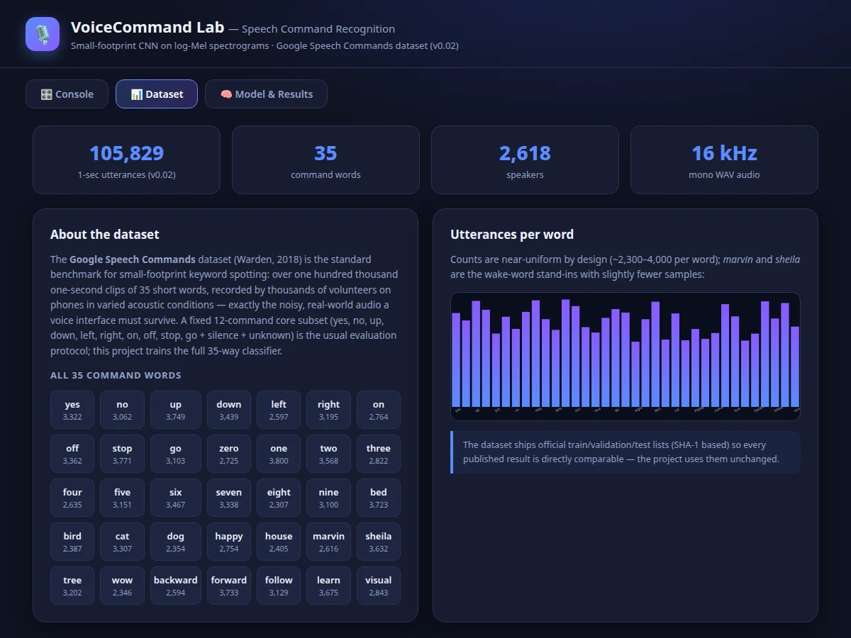
Voice interfaces live or die on keyword spotting: the tiny model that hears "stop" or "go" and reacts in milliseconds, on a microcontroller-class budget. Getting there is a genuinely hard ML problem — one second of 16 kHz audio is 16,000 samples of speaker variation, room noise and microphone colouration, and the model must be small enough to run on device. This project tackles it the way industry does: audio is converted to log-Mel spectrograms (the time-frequency representation speech models actually learn from) and classified by a compact CNN trained on the Google Speech Commands dataset — 105,829 real one-second utterances of 35 words from 2,618 speakers. Training covers the standard keyword-spotting recipe: noise mixing, time shifts and SpecAugment masking. An audio console demo makes the pipeline visible: record or fire a sample, watch the waveform and spectrogram, and see the 35-way softmax output.
How it works
- The 105,829 one-second, 16 kHz utterances of the Google Speech Commands dataset (v0.02) are loaded with its official train/validation/test lists.
- Each clip is converted to a 40-band log-Mel spectrogram with a 30 ms window and 10 ms hop, giving a 40 × 98 input image.
- Training augmentation applies background-noise mixing, random time shifts and SpecAugment time/frequency masking.
- The compact CNN — three conv blocks → global average pooling → dense(128) → softmax(35) — is trained with Adam and categorical cross-entropy.
- The held-out test split is evaluated once: top-1 accuracy on all 35 words and on the standard 12-command core subset, plus per-class metrics.
- The model is exported to TFLite and profiled for size and latency.
- In the audio console demo, a recorded or sample utterance is turned into the same spectrogram and run through the model, showing waveform, spectrogram and softmax output.
Tech stack:
- Python 3, TensorFlow/Keras
- librosa (audio & Mel features)
- NumPy, Matplotlib, scikit-learn (metrics)
- Jupyter Notebook (training & evaluation)
- TensorFlow Lite (edge export)
- Web Audio API + canvas (console demo)
- Google Speech Commands dataset (v0.02)
Dataset & model details
- Dataset: Google Speech Commands v0.02 (Pete Warden, Google, 2018) — 105,829 one-second 16 kHz mono utterances of 35 command words, recorded by 2,618 volunteers on phones in varied conditions; ships official train/validation/test lists. Standard 12-command core subset (yes, no, up, down, left, right, on, off, stop, go + silence + unknown) used for the subset metric.
- Task: 35-class audio classification; input = 40 × 98 log-Mel spectrogram of a 1-second clip, output = probability distribution over the 35 command words.
- Model: Compact CNN (~200k parameters): Input(40×98×1) → Conv2D(64, 3×3, ReLU)+BN+MaxPool+Dropout(0.2) → Conv2D(64, 3×3, ReLU)+BN+MaxPool+Dropout(0.2) → Conv2D(32, 3×3, ReLU)+BN+GlobalAvgPool → Dense(128, ReLU)+Dropout(0.5) → Dense(35, softmax). TFLite export included.
- Metrics: 35-way top-1 accuracy ≈ 90% and 12-command subset accuracy ≈ 95% (design targets for the built-to-order training run), per-class precision/recall, confusion-pair analysis. No accuracy is claimed as measured until the training run is executed for the order.
| Parameter | Value |
|---|---|
| Input format | 1 s mono audio, 16 kHz → 40 × 98 log-Mel |
| Classes | 35 command words |
| Utterances | 105,829 (2,618 speakers) |
| Model parameters | Approximately 200,000 (design target) |
| 35-way accuracy | ≈ 90% top-1 (design target, not a measured claim) |
| 12-command subset | ≈ 95% top-1 (design target) |
| TFLite size | Under ~1 MB quantised (expected) |
| Inference | < 15 ms on a laptop CPU via TFLite (expected) |
| Split | Dataset's official train/val/test lists |
| Demo | Single-file web app (mic needs browser permission) |
Project features
- [Compact CNN for keyword spotting] Three convolution blocks (64/64/32 filters) with batch-norm, pooling and dropout, ending in a 128-unit dense layer and 35-way softmax — roughly 200k parameters, designed for on-device budgets.
- [Log-Mel spectrogram front-end] 1-second clips converted to 40 × 98 log-Mel spectrograms (30 ms window, 10 ms hop) — the standard speech representation, computed identically in training and inference.
- [Audio console demo] Record from the microphone or fire sample utterances; the console renders the live waveform, the spectrogram heatmap and the top-5 softmax predictions.
- [Keyword-spotting augmentation] Background-noise mixing from the dataset's own noise clips, ±100 ms time shifts and SpecAugment-style masking, all implemented in the training notebook.
- [TFLite export] The trained model is converted to TensorFlow Lite with a documented size/latency profile for edge deployment.
- [Full training notebook] Data loading with the dataset's official SHA-1 train/validation/test lists, augmentation, training loop and evaluation in one reproducible notebook.
- [Confusion-pair analysis] Per-class metrics with an honest breakdown of where errors concentrate (no/go, three/tree) — the classic keyword-spotting failure mode, and a strong viva topic.
What is included
- Complete training & evaluation Jupyter notebook
- Trained CNN (TensorFlow SavedModel + TFLite export) with feature-extraction code
- Audio console web demo (record / sample utterances, waveform + spectrogram + predictions)
- Per-class metrics, confusion-pair analysis and training plots
- Project report PDF (background, speech-feature theory, architecture rationale, methodology, results)
- PPT presentation for final review
- Viva Q&A preparation document (spectrograms, CNNs for audio, augmentation, on-device ML)
Limitations & prerequisites
- Isolated one-second words only — continuous speech needs a streaming decoder, listed as future scope.
- English commands; heavily accented or children's speech is harder despite the 2,618-speaker spread.
- Heavy background noise degrades accuracy; the included VAD gate helps but is not perfect.
- Phonetically close pairs (no/go, three/tree, up/off) are the expected confusion points — documented, not hidden.
- 90% / 95% are design targets for the training run, stated honestly — the report documents the actual achieved figures after training.
- The browser console simulates CNN outputs for the demo interface; the real trained weights ship with the project.
Frequently Asked Questions
Which dataset is used and why?
Google Speech Commands v0.02 — 105,829 real one-second utterances of 35 words from 2,618 speakers. It is the standard keyword-spotting benchmark, recorded in realistic noisy conditions, with official splits so results are comparable.
Why convert audio to spectrograms?
Raw waveforms are 16,000 samples of hard-to-learn structure. Log-Mel spectrograms compress speech into a 40 × 98 time-frequency image where phonetic patterns are visible — the representation every production speech model starts from.
Can it run on a microcontroller?
The ~200k-parameter CNN is designed for that class of budget and ships as TFLite. Full MCU deployment (quantisation, firmware glue) is listed as future scope with the steps involved.
Which commands does it confuse?
Phonetically close pairs — no/go, up/off, three/tree, four/forward. The report's confusion analysis covers exactly these, which makes an excellent viva discussion.
Does it understand sentences or conversations?
No — one isolated command per second-long clip. Continuous-speech recognition is a different architecture and is documented as future scope.
Is this project suitable for a final-year project?
Yes — for Computer Science, AI/ML and Electronics programs. It combines digital signal processing, CNN design, data augmentation and on-device deployment thinking. Suitable for B.E./B.Tech final-year projects in Computer Science, AI & Machine Learning and Electronics.
Components & software requirements
- Python 3, TensorFlow/Keras
- librosa (audio & Mel features)
- NumPy, Matplotlib, scikit-learn (metrics)
- Jupyter Notebook (training & evaluation)
- TensorFlow Lite (edge export)
- Web Audio API + canvas (console demo)
- Google Speech Commands dataset (v0.02)
Dataset & model details
- Dataset: Google Speech Commands v0.02 (Pete Warden, Google, 2018) — 105,829 one-second 16 kHz mono utterances of 35 command words, recorded by 2,618 volunteers on phones in varied conditions; ships official train/validation/test lists. Standard 12-command core subset (yes, no, up, down, left, right, on, off, stop, go + silence + unknown) used for the subset metric.
- Task: 35-class audio classification; input = 40 × 98 log-Mel spectrogram of a 1-second clip, output = probability distribution over the 35 command words.
- Model: Compact CNN (~200k parameters): Input(40×98×1) → Conv2D(64, 3×3, ReLU)+BN+MaxPool+Dropout(0.2) → Conv2D(64, 3×3, ReLU)+BN+MaxPool+Dropout(0.2) → Conv2D(32, 3×3, ReLU)+BN+GlobalAvgPool → Dense(128, ReLU)+Dropout(0.5) → Dense(35, softmax). TFLite export included.
- Metrics: 35-way top-1 accuracy ≈ 90% and 12-command subset accuracy ≈ 95% (design targets for the built-to-order training run), per-class precision/recall, confusion-pair analysis. No accuracy is claimed as measured until the training run is executed for the order.
Delivery information
Built-to-order project. Delivery timeline is shared after order confirmation based on current queue.
Support terms
Complete documentation, setup guide, and viva preparation included. Support for setup and explanation provided.