
More project photos (3)
The problem
Land-use maps are normally drawn by analysts who inspect satellite imagery patch by patch, a process that is slow, subjective and hard to repeat over large areas or over time. Two neighbouring patches can look deceptively similar from orbit — pasture and herbaceous vegetation, or annual and permanent crops, often differ only in texture, field pattern and seasonal colour — so manual labelling does not scale and different labellers disagree. This project automates that first pass with a convolutional neural network trained on the EuroSAT benchmark: each Sentinel-2 patch is classified into one of 10 land-use classes, with per-class probabilities so uncertain patches can be flagged for human review instead of silently accepted. The full pipeline, from data loading to confusion-matrix evaluation, is documented so the student can explain every decision.
27,000 labelled Sentinel-2 patches, 64x64 RGB, in 10 land-use classes.
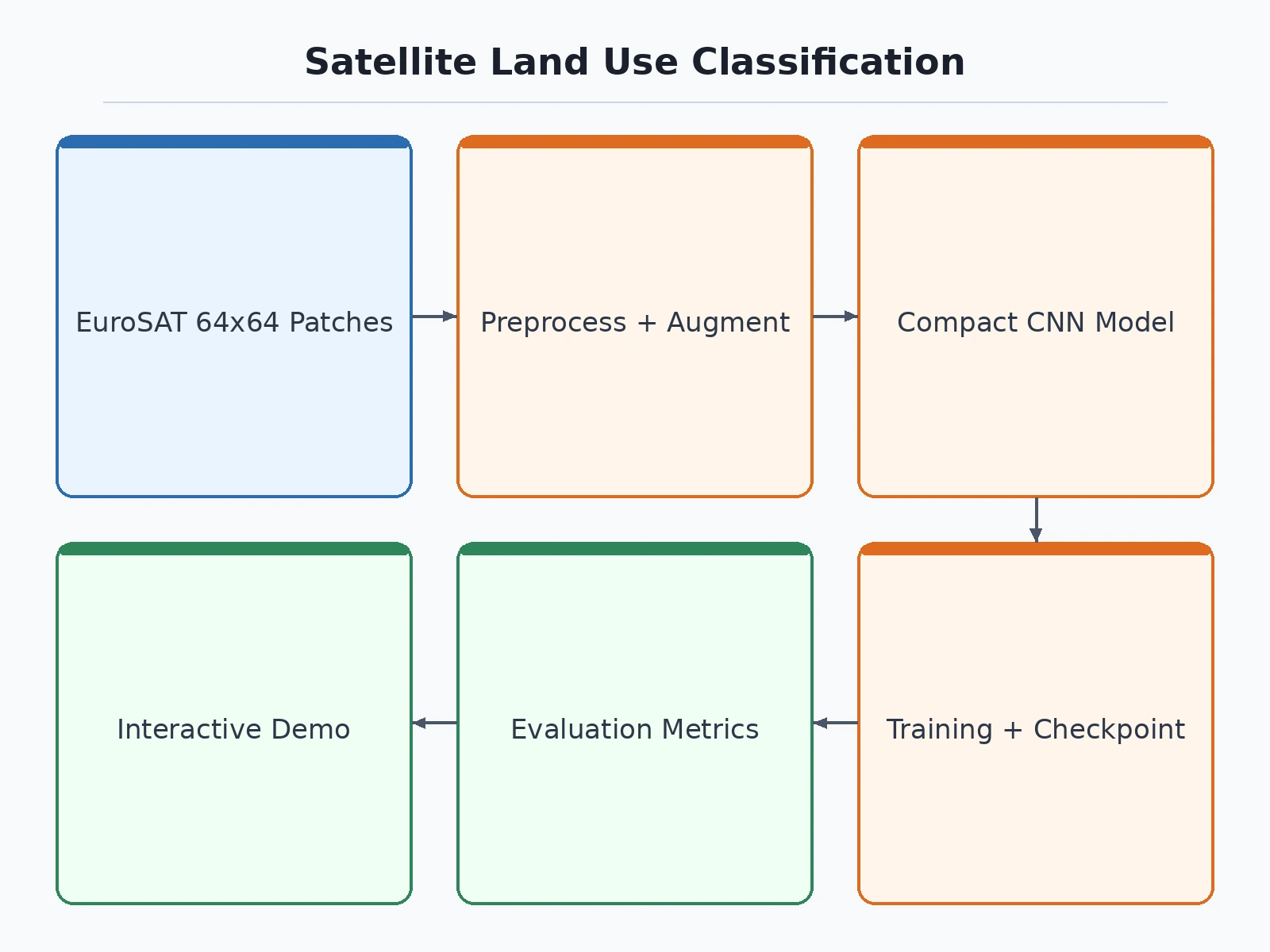
Follow the working sequence
How it works
- Dataset: The EuroSAT RGB dataset is loaded — Sentinel-2 patches of 64×64 pixels in 10 land-use classes — and split with stratification into training, validation and test subsets.
- Preprocessing: Patches are normalised to the range [0, 1], and training patches receive light augmentation (flips and small rotations) because satellite views have no fixed orientation.
- Training: The compact CNN — convolution blocks with ReLU and max-pooling, dropout, a dense layer and a softmax output over 10 classes — is trained with the Adam optimiser and categorical cross-entropy loss.
- Evaluation: The held-out test subset is evaluated once, producing overall accuracy, per-class precision, recall and F1-score, and the full confusion matrix for the report.
- Inference: A new patch is resized to 64×64 pixels, normalised exactly as in training, and passed through the saved model to obtain a probability for every class.
- Output: The demo and report present the top predicted class, the complete probability distribution and the ground-truth label where available, so errors can be inspected patch by patch.
Tech stack:
- Python 3, TensorFlow/Keras
- EuroSAT dataset (Sentinel-2 imagery)
- NumPy, Matplotlib
- scikit-learn (metrics and splits)
- Jupyter Notebook (training and evaluation)
- HTML, CSS and JavaScript (interactive demo)
Dataset & model details
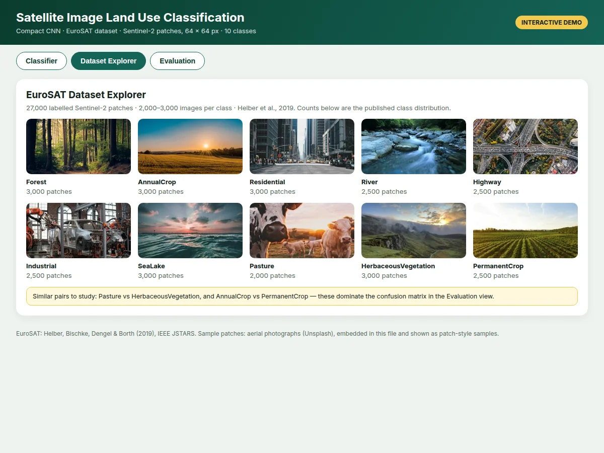
- Dataset: EuroSAT (Helber et al., 2019) — 27,000 labelled Sentinel-2 satellite image patches, each 64×64 pixels, in 10 land-use and land-cover classes with 2,000 to 3,000 images per class (design target split: stratified training, validation and test subsets). This project uses the RGB version of the dataset; the original release also provides 13 spectral bands. Classes: AnnualCrop, Forest, HerbaceousVegetation, Highway, Industrial, Pasture, PermanentCrop, Residential, River, SeaLake.
- Task: 10-class single-label image classification; input = one 64×64×3 RGB satellite patch, output = probability distribution over the 10 land-use classes, with the highest-probability class taken as the prediction.
- Model: Compact custom CNN: Conv2D (32 filters) → MaxPool → Conv2D (64 filters) → MaxPool → Conv2D (128 filters) → MaxPool → Dropout → Flatten → Dense → Dropout → Dense with softmax over 10 classes, trained with Adam and categorical cross-entropy. A transfer-learning baseline is discussed in the report as a comparison option, not as the shipped model.
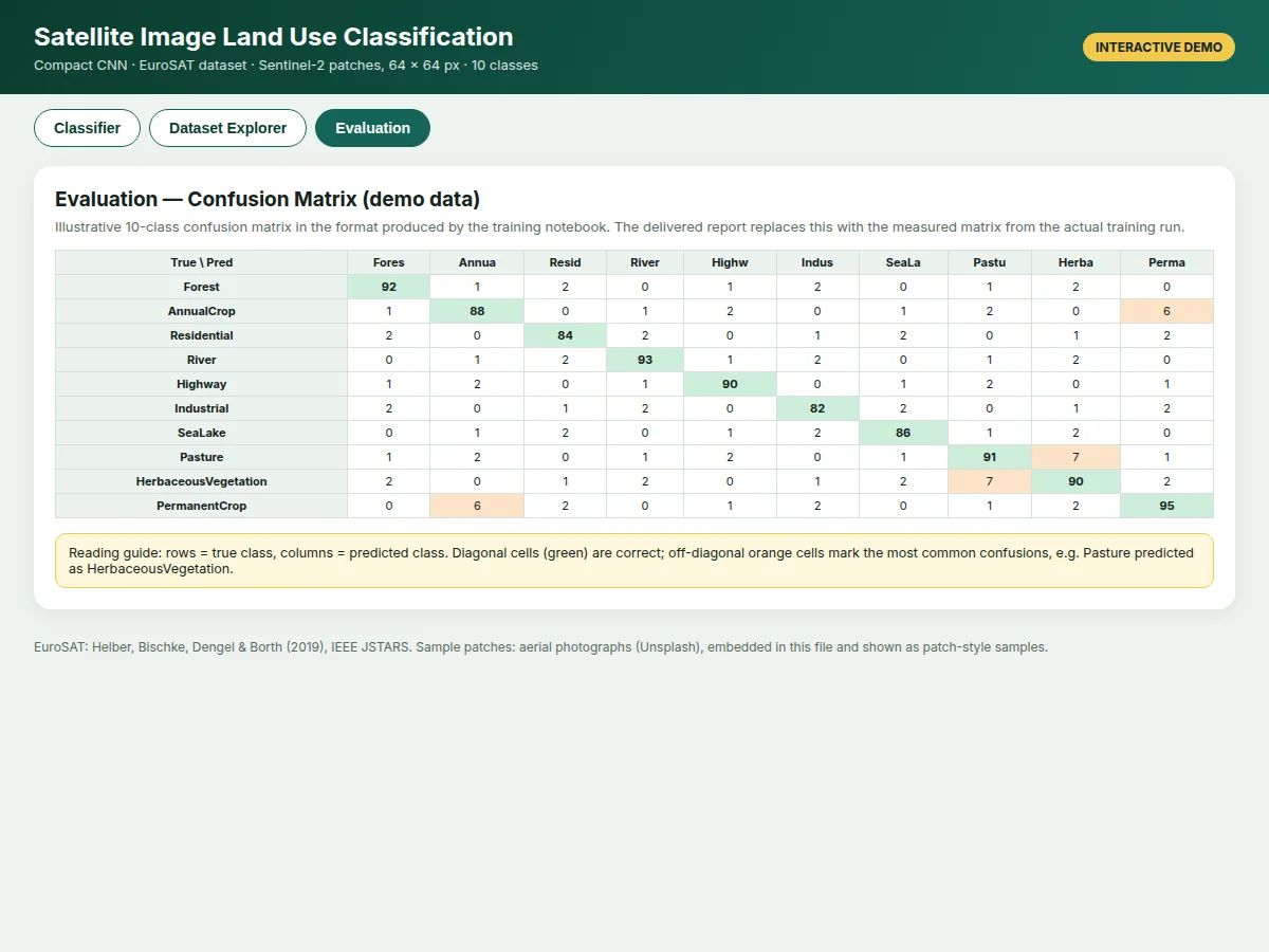
- Metrics: Overall accuracy (design target only — see Specifications), per-class precision, recall and F1-score, and a 10×10 confusion matrix on the held-out test subset. No accuracy figure is claimed as measured until the training run for the order is executed and documented.
| Parameter | Value |
|---|---|
| Input format | 64 × 64 pixels RGB, normalised to [0, 1] (dataset specification) |
| Dataset size | 27,000 images approx. (dataset specification) |
| Classes | 10 classes (dataset specification) |
| Images per class | 2,000 to 3,000 images per class (dataset specification) |
| Model parameters | Approximately 500,000 parameters (design target) |
| Test accuracy | Approximately 90% (design target, not a measured claim) |
| Training time | Approximately 30 to 60 minutes on a GPU notebook (expected) |
| Inference time | Under 1 second per patch on CPU (expected) |
| Model file size | Approximately 2 MB to 5 MB (expected) |
| Demo | Single-file web app, runs in browser (design target) |
Project features
- [Compact custom CNN classifier] Three convolution–pooling blocks followed by dense layers and a softmax output, designed for small 64×64 patches so training stays feasible on a laptop or free GPU notebook.
- [EuroSAT dataset explorer] Browse example patches and counts for all 10 classes, so the class definitions and the visual differences between similar classes are understood before training begins.
- [Interactive classification demo] Select a sample patch and view the predicted land-use class with the full per-class probability distribution, honestly labelled as demo data in the web preview.
- [Confusion matrix and per-class report] Precision, recall and F1-score per class plus a 10×10 confusion matrix, so confusions such as Pasture versus HerbaceousVegetation can be discussed with evidence.
- [Reproducible training notebook] Data loading, stratified splitting, augmentation, model definition, training and evaluation in one notebook with every hyperparameter recorded and explained.
- [Training curves and checkpointing] Accuracy and loss plots for training versus validation, with the best weights checkpointed on validation accuracy rather than the final epoch.
- [Exported model with preprocessing code] Saved model weights bundled with the exact resizing and normalisation pipeline, so inference in the demo matches training-time preprocessing.
What is included
- Complete training and evaluation Jupyter notebook
- Trained CNN model file with preprocessing code
- Interactive classification and dataset-explorer web demo
- Confusion matrix, per-class metrics and training-curve plots
- Project report PDF (background, dataset, architecture, methodology, results)
- PPT presentation for final review
- Viva Q&A preparation document (CNN design, EuroSAT classes, evaluation metrics)
Limitations & prerequisites
- Trained only on European Sentinel-2 patches from EuroSAT — land cover in other regions, seasons or sensors may look different and reduce accuracy (expected).
- Similar classes are genuinely confusable, notably Pasture versus HerbaceousVegetation and AnnualCrop versus PermanentCrop; the confusion matrix documents this rather than hiding it.
- The approximately 90% accuracy figure is a design target for the training run, not a measured result — the report records the figure actually achieved.
- Each patch receives exactly one label, even where a patch visibly mixes two land uses, because EuroSAT itself is single-label.
- The RGB version discards the additional spectral bands available in the original multispectral release, which can help separate vegetation types.
- This is an academic classification prototype, not a certified land-survey or planning product, and its maps should not be used for legal or regulatory decisions.
Frequently Asked Questions
Which dataset is used and why?
EuroSAT, released by Helber and colleagues, contains 27,000 labelled Sentinel-2 patches in 10 land-use classes at 64×64 pixels. It is the standard benchmark for this task: small enough to train on modest hardware, openly available, and directly comparable with published results, which makes methodology and evaluation easy to defend.
Which model is used and what does it output?
A compact custom CNN with three convolution–pooling blocks, dropout and a softmax output layer. It takes one 64×64 RGB patch as input and outputs a probability for each of the 10 classes. The predicted class is the highest-probability one, and the full distribution is always shown so low-confidence predictions are visible.
Is the accuracy guaranteed?
No. The figure in the specifications is a design target for the training run, stated honestly as such. Actual accuracy depends on the split, augmentation, hyperparameters and training duration. The delivered report documents the measured test accuracy, per-class precision, recall and F1-score, and the confusion matrix from the actual run.
Can new classes or a custom area be added?
EuroSAT covers 10 fixed classes, so a new class needs labelled patches for that class and a retraining run; the notebook is structured to allow this. Classifying imagery of a specific local area is possible as an optional customisation if labelled examples are supplied, but accuracy there is not covered by the EuroSAT evaluation.
Does the demo run the real trained model?
The delivered demo is wired to the exported model and its preprocessing pipeline. The hosted preview on this page uses clearly labelled demo data to illustrate the interface without loading model weights in the browser, so preview probabilities should be read as illustrative, not as live model outputs.
Is this project suitable for a final-year project?
Yes — for AI & Machine Learning, Computer Science and IT programmes. It demonstrates dataset handling for remote-sensing imagery, CNN design for small images, augmentation, disciplined train, validation and test evaluation, and error analysis through a confusion matrix, all of which support a well-evidenced final review discussion.
Components & software requirements
- Python 3, TensorFlow/Keras
- EuroSAT dataset (Sentinel-2 imagery)
- NumPy, Matplotlib
- scikit-learn (metrics and splits)
- Jupyter Notebook (training and evaluation)
- HTML, CSS and JavaScript (interactive demo)
Dataset & model details
- Dataset: EuroSAT (Helber et al., 2019) — 27,000 labelled Sentinel-2 satellite image patches, each 64×64 pixels, in 10 land-use and land-cover classes with 2,000 to 3,000 images per class (design target split: stratified training, validation and test subsets). This project uses the RGB version of the dataset; the original release also provides 13 spectral bands. Classes: AnnualCrop, Forest, HerbaceousVegetation, Highway, Industrial, Pasture, PermanentCrop, Residential, River, SeaLake.
- Task: 10-class single-label image classification; input = one 64×64×3 RGB satellite patch, output = probability distribution over the 10 land-use classes, with the highest-probability class taken as the prediction.
- Model: Compact custom CNN: Conv2D (32 filters) → MaxPool → Conv2D (64 filters) → MaxPool → Conv2D (128 filters) → MaxPool → Dropout → Flatten → Dense → Dropout → Dense with softmax over 10 classes, trained with Adam and categorical cross-entropy. A transfer-learning baseline is discussed in the report as a comparison option, not as the shipped model.
- Metrics: Overall accuracy (design target only — see Specifications), per-class precision, recall and F1-score, and a 10×10 confusion matrix on the held-out test subset. No accuracy figure is claimed as measured until the training run for the order is executed and documented.
Delivery information
Built-to-order project. Delivery timeline is shared after order confirmation based on current queue.
Support terms
Complete documentation, setup guide, and viva preparation included. Support for setup and explanation provided.
Download free synopsis (PDF)
Enter your name and email — the synopsis PDF downloads immediately. We may send occasional project updates; no spam, unsubscribe anytime.