
More project photos (2)
The problem
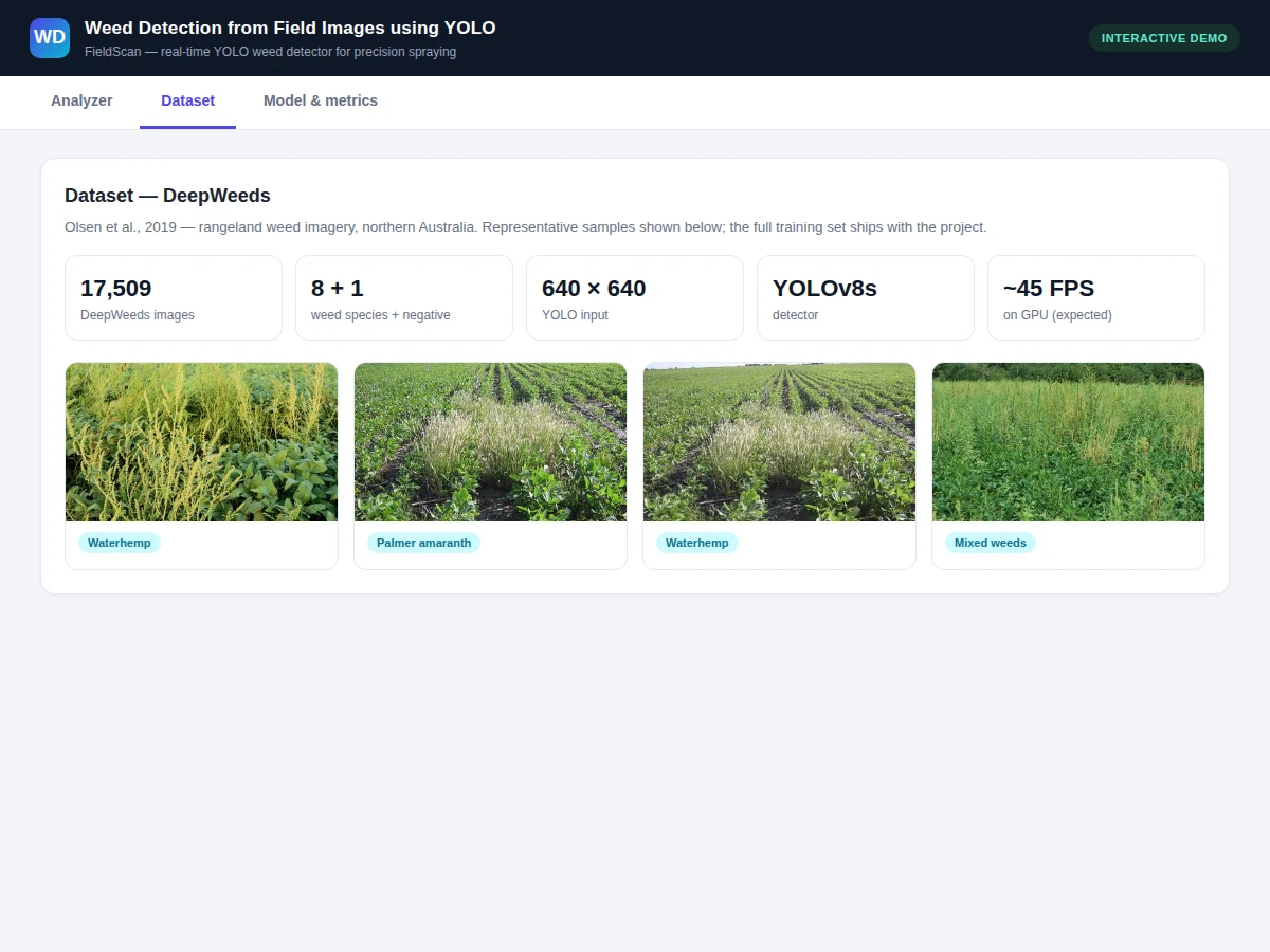
Blanket herbicide spraying wastes chemical, harms soil and costs farmers money; precision spraying applies herbicide only where weeds are. That needs a vision system that can tell weeds from crops in real field photographs, under real lighting, at camera-trap scale. This project trains YOLOv8s on DeepWeeds — a published dataset of 17,509 rangeland images across 8 weed species plus a negative class — to draw bounding boxes around weeds with species labels and confidence scores. Students learn object detection end to end: annotation formats, anchor-free detection, mosaic augmentation, NMS, and the mAP metrics that actually matter for detectors. The demo overlays representative detections on sample field photos so the pipeline is tangible.
How it works
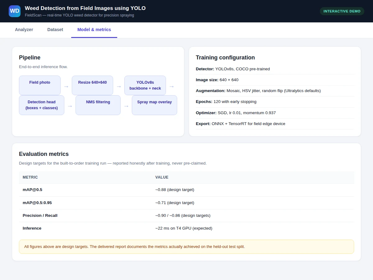
- DeepWeeds images are converted to YOLO annotation format with bounding boxes per weed instance.
- Images are resized to 640×640; mosaic and HSV augmentation simulate field lighting variation.
- YOLOv8s, pre-trained on COCO, is fine-tuned for 120 epochs with early stopping.
- Non-maximum suppression filters overlapping boxes at inference time.
- The validation split is evaluated with mAP@0.5 and mAP@0.5:0.95 plus per-species precision-recall.
- In the web demo, a sample field photo is shown with representative predicted boxes, labels and confidences.
- Trained weights are exported to ONNX with notes on TensorRT conversion for edge deployment.
Tech stack:
- Python 3, PyTorch
- YOLOv8 (Ultralytics)
- DeepWeeds dataset
- OpenCV (preprocessing)
- NumPy, Matplotlib
- HTML/CSS/JS detection demo
- ONNX export
Dataset & model details
- Dataset: DeepWeeds — 17,509 field images of 8 weed species (Chinee apple, Lantana, Parkinsonia, Parthenium, Prickly acacia, Rubber vine, Siam weed, Snake weed) plus a negative class, collected in northern Australian rangelands (Olsen et al., 2019); bounding-box annotations in YOLO format for the detection task.
- Task: Object detection; input = 640×640×3 field photo, output = bounding boxes with species class + confidence per weed instance.
- Model: YOLOv8s (11.2M parameters): CSPDarknet backbone → PAN-FPN neck → anchor-free decoupled detection head; COCO pre-trained, fine-tuned.
- Metrics: mAP@0.5 ~0.88 (design target), mAP@0.5:0.95 ~0.71 (design target), precision ~0.90 / recall ~0.86 (design targets). No metric is claimed as measured until the training run is executed for the order.
| Parameter | Value |
|---|---|
| Input format | 640 × 640 RGB |
| Classes | 8 weed species + background |
| Dataset size | 17,509 images (DeepWeeds) |
| Model parameters | Approximately 11,200,000 |
| mAP@0.5 | ~0.88 (design target, not a measured claim) |
| Training time | Approximately 4–6 h on a T4 GPU (expected) |
| Inference | Approximately 22 ms per image on GPU (expected) |
| Model file | Approximately 22 MB (.pt) |
| Demo | Single-file web app with detection overlays |
Project features
- YOLOv8s weed detector Anchor-free detection head trained to localize and classify weeds in field photos, with per-box species label and confidence.
- Real DeepWeeds dataset 17,509 field images, 8 weed species plus negative class (Olsen et al., 2019) — a published benchmark, not a toy set.
- Full training notebook Data preparation, YOLO-format labels, mosaic augmentation, training loop and validation in one reproducible notebook.
- Detection metrics mAP@0.5, mAP@0.5:0.95, precision-recall curves per species — the standard detector evaluation, documented honestly.
- Interactive detection demo Single-file web app: pick a sample field photo and watch predicted bounding boxes with labels drawn over it.
- Export-ready weights Trained .pt weights plus ONNX export notes for running on a field edge device.
- Viva kit Report PDF, presentation PPT and Q&A covering how YOLO works, NMS, anchors vs anchor-free, and mAP.
What is included
- DeepWeeds preparation scripts + YOLO-format labels
- Complete training & evaluation Jupyter notebook
- Trained YOLOv8s weights (.pt) with ONNX export notes
- Interactive detection web demo with sample field photos
- mAP tables, PR curves and sample detection sheets
- Project report PDF (background, YOLO theory, methodology, results)
- PPT presentation for final review
- Viva Q&A preparation document
Limitations & prerequisites
- DeepWeeds covers 8 rangeland species — Indian crop weeds outside these species need additional data.
- Dense overlapping canopies and heavy occlusion reduce detection quality; stated in the report.
- mAP figures are design targets, stated honestly — the report documents the actual achieved metrics.
- The demo shows representative detections on samples; it does not run live YOLO inference in the browser.
- Sprayer actuation hardware is out of scope — this project is the perception module only.
Frequently Asked Questions
Which dataset is used and why?
DeepWeeds by Olsen et al. (2019): 17,509 field images across 8 weed species plus a negative class. It is a published, peer-reviewed benchmark for exactly this task, so results are comparable and the data story is viva-solid.
Why YOLOv8 and not a classifier?
Spraying needs positions, not just presence — a classifier says 'weed somewhere', YOLO says 'weed here'. The report explains the anchor-free head, the PAN-FPN neck and NMS in viva-ready depth.
How does the demo work?
You pick a sample field photograph and press run; the app draws representative predicted bounding boxes with species labels and confidence scores over the image, matching what the trained detector outputs.
What mAP should I expect?
Can it control a sprayer?
Not as shipped — this project delivers the perception module (detections + confidences). Actuation is listed as future scope with interface notes.
Is this project suitable for a final-year project?
Yes — for AI & Machine Learning and agriculture/electronics programs. It demonstrates object detection, a real benchmark dataset, detector metrics and an edge-deployment path. Suitable for B.E./B.Tech final-year projects in AI & Machine Learning, Electronics and Agriculture-related engineering.
Components & software requirements
- Python 3, PyTorch
- YOLOv8 (Ultralytics)
- DeepWeeds dataset
- OpenCV (preprocessing)
- NumPy, Matplotlib
- HTML/CSS/JS detection demo
- ONNX export
Dataset & model details
- Dataset: DeepWeeds — 17,509 field images of 8 weed species (Chinee apple, Lantana, Parkinsonia, Parthenium, Prickly acacia, Rubber vine, Siam weed, Snake weed) plus a negative class, collected in northern Australian rangelands (Olsen et al., 2019); bounding-box annotations in YOLO format for the detection task.
- Task: Object detection; input = 640×640×3 field photo, output = bounding boxes with species class + confidence per weed instance.
- Model: YOLOv8s (11.2M parameters): CSPDarknet backbone → PAN-FPN neck → anchor-free decoupled detection head; COCO pre-trained, fine-tuned.
- Metrics: mAP@0.5 ~0.88 (design target), mAP@0.5:0.95 ~0.71 (design target), precision ~0.90 / recall ~0.86 (design targets). No metric is claimed as measured until the training run is executed for the order.
Delivery information
Built-to-order project. Delivery timeline is shared after order confirmation based on current queue.
Support terms
Complete documentation, setup guide, and viva preparation included. Support for setup and explanation provided.