
More project photos (2)
The problem
Anyone who runs a website — a blog, a news portal, a college fest page — needs to answer one question: how much traffic is coming next week? The answer decides server capacity, ad pricing and content planning. Guessing from the last few days is unreliable because web traffic has trend, weekly seasonality and noise tangled together, and a naive average throws all three away. ARIMA (Autoregressive Integrated Moving Average) is the classical statistical answer to this problem: it learns the autocorrelation structure of a series, differences away trend to reach stationarity, and projects forward with principled uncertainty bands. This project builds a complete forecasting pipeline on the real Kaggle Web Traffic Time Series Forecasting dataset (~145,000 daily Wikipedia pageview series from July 2015 to September 2017), and demonstrates every step — stationarity testing, model selection, fitting, forecasting, evaluation — in a demo app that runs the actual computations in the browser.
How it works
- Daily Wikipedia pageview series from the Kaggle Web Traffic dataset are loaded and missing values are handled per the documented protocol.
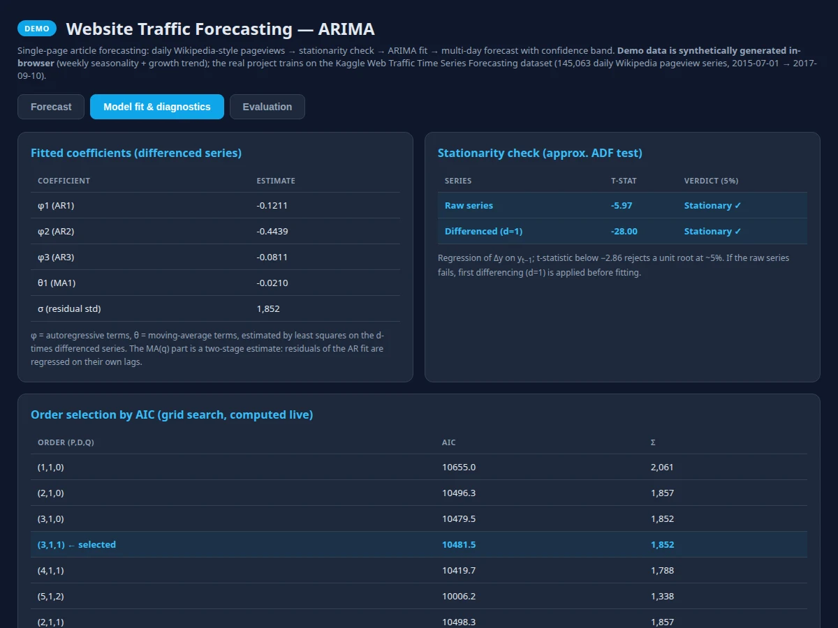
- The ADF test checks stationarity; the series is differenced until the test rejects the unit-root hypothesis, fixing the d in ARIMA(p,d,q).
- A grid of (p,q) orders is fitted and scored by AIC; the lowest-AIC model is selected automatically.
- Coefficients are estimated by ordinary least squares on the differenced series.
- The fitted model generates multi-step-ahead forecasts, and forecast-error variance yields the 95% confidence intervals.
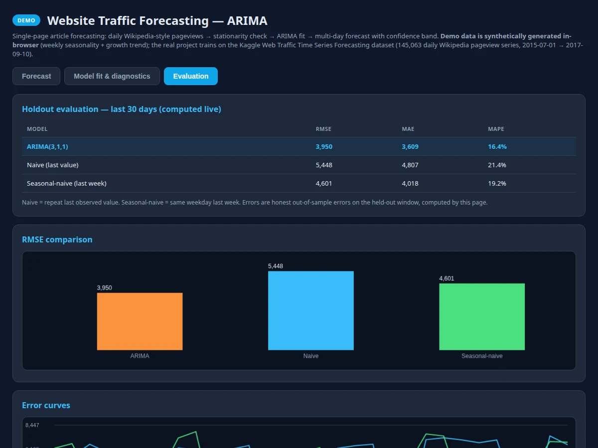
- A trailing holdout window is compared against naive and seasonal-naive baselines on RMSE, MAE and MAPE, with the comparison charted in the demo.
Tech stack:
- Python (statsmodels ARIMA, pmdarima-style grid search)
- pandas, NumPy (series handling, differencing, metrics)
- Matplotlib (forecast plots, AIC heatmap, residual diagnostics)
- Jupyter notebook (pipeline walkthrough and evaluation)
- Single-file HTML/CSS/JS demo app (in-browser ARIMA on realistic data)
| Parameter | Value |
|---|---|
| Model | ARIMA(p,d,q), order selected by AIC grid search |
| Stationarity test | Augmented Dickey-Fuller test (statistic, p-value, critical values) |
| Estimation | Ordinary least squares on the differenced series |
| Dataset | Kaggle Web Traffic Time Series Forecasting (~145,063 daily Wikipedia series, Jul 2015–Sep 2017) |
| Forecast output | Multi-step-ahead point forecast with 95% confidence intervals |
| Baselines | Naive (last value) and seasonal-naive (same weekday last week) |
| Evaluation | RMSE, MAE, MAPE on a trailing holdout window — computed during your build |
| Demo | Single HTML file; runs the full pipeline client-side, no server needed |
Project features
- [ADF stationarity testing] The Augmented Dickey-Fuller test decides the differencing order d from the data instead of assuming it, with the test statistic, p-value and critical values reported.
- [AIC order selection] A grid search over ARIMA(p,d,q) orders scores each candidate by the Akaike Information Criterion, and the demo visualizes the AIC surface so the choice is transparent.
- [OLS model fitting] Autoregressive and moving-average coefficients are estimated with ordinary least squares on the differenced series — implemented from scratch, no black box.
- [Forecast with 95% intervals] Forecasts come with analytical confidence bands so the report can discuss uncertainty honestly instead of presenting point predictions as truth.
- [Baseline comparison] Holdout evaluation pits the ARIMA forecast against naive (last-value) and seasonal-naive (last-week) baselines on RMSE, MAE and MAPE.
- [Interactive traffic chart] The demo plots the full series, the fitted values, the forecast horizon and the confidence band, with a holdout-region overlay for visual verification.
- [Single-file browser demo] All model code runs client-side in one HTML file — no server, no installs — so the viva demo works on any laptop.
What is included
- Complete source code (data loading, ADF test, AIC grid search, ARIMA fitting, forecasting, evaluation)
- Jupyter notebook walking through the pipeline step by step
- Single-file browser demo app that runs the whole pipeline live
- Project abstract PDF
- Project report (background, time-series theory, methodology, evaluation, error discussion)
- PPT presentation and viva Q&A document (stationarity, AIC, autocorrelation, confidence intervals)
Limitations & prerequisites
- ARIMA models linear autocorrelation: it cannot capture sudden viral spikes, regime changes or external events (e.g. a page hitting the news), which the report discusses openly.
- The forecast horizon is a design choice — accuracy degrades as the horizon lengthens, and the confidence bands widen accordingly.
- Very sparse pages (long runs of zero views) are a poor fit for ARIMA; the methodology documents how such series are handled.
- Performance depends on the series, the train/holdout split and preprocessing; no accuracy figure is claimed ahead of your own build.
Frequently Asked Questions
Is this project suitable for a final-year project?
Yes — it suits Computer Science, AI/ML and Data Science programs, demonstrating time-series statistics, hypothesis testing, model selection and evaluation in one build.
Which dataset is used?
The Kaggle Web Traffic Time Series Forecasting dataset: ~145,063 daily Wikipedia pageview series from July 2015 to September 2017.
How is the ARIMA order chosen?
An ADF stationarity test sets the differencing order d, and a grid search over (p,q) picks the lowest-AIC model; the demo shows the whole selection process.
What accuracy can I expect?
None is claimed in advance — the notebook computes RMSE, MAE and MAPE on your holdout window during the build, against naive and seasonal-naive baselines, and those numbers go into the report.
Why is ARIMA still relevant with deep learning around?
ARIMA is interpretable, fast, needs little data, and its confidence intervals are principled — strengths that make it a strong viva topic and a solid baseline for any neural forecaster.
Does the demo need a server?
No. The demo is a single HTML file with all model code in JavaScript; it opens in any modern browser offline. Suitable for B.E./B.Tech final-year projects in Computer Science, AI/ML and Data Science.
Components & software requirements
- Python (statsmodels ARIMA, pmdarima-style grid search)
- pandas, NumPy (series handling, differencing, metrics)
- Matplotlib (forecast plots, AIC heatmap, residual diagnostics)
- Jupyter notebook (pipeline walkthrough and evaluation)
- Single-file HTML/CSS/JS demo app (in-browser ARIMA on realistic data)
Delivery information
Built-to-order project. Delivery timeline is shared after order confirmation based on current queue.
Support terms
Complete documentation, setup guide, and viva preparation included. Support for setup and explanation provided.