
More project photos (2)
The problem
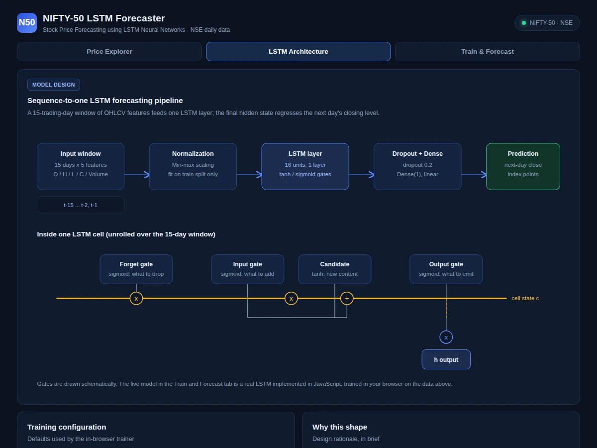
Stock-price prediction is one of the most picked — and most poorly executed — final-year ML topics. Typical builds shuffle time-series data before splitting (leaking the future into training), report a single accuracy-style number with no baseline, and collapse the moment an examiner asks why the model should beat "tomorrow looks like today". This project takes the disciplined route: real NIFTY-50 daily OHLCV data from the NSE, strictly chronological splits, scalers fit on training data only, and a persistence baseline running on the same evaluation folds so the model's true edge is explicit. A sequence-to-one LSTM learns from 15-day windows of open, high, low, close and volume to regress the next day's closing level, evaluated with RMSE, MAE and MAPE under walk-forward retraining. A live web demo makes the whole pipeline tangible: the price explorer charts the real series, and a pure-JavaScript LSTM trains in the browser while loss curves and forecast-vs-actual plots update live.
How it works
- Daily OHLCV for NIFTY-50 (^NSEI) is fetched from NSE archives via yfinance — 249 trading days (27 Sep 2024 – 26 Sep 2025) in the reference build.
- Each training sample becomes a 15-day window of 5 features (open, high, low, close, volume); the target is the next trading day's close.
- The series is split chronologically 80/20 with no shuffling, and min-max scalers are fit on the training portion only.
- A Keras model — LSTM(32) → Dropout(0.2) → Dense(1, linear) — trains with Adam (learning rate 0.005) on mean squared error, with early stopping on a validation slice.
- Walk-forward evaluation retrains on an expanding window and scores each held-out fold with RMSE, MAE and MAPE.
- The persistence baseline (predict yesterday's close) is scored on the identical folds, so any edge — or lack of one — is stated plainly in the report.
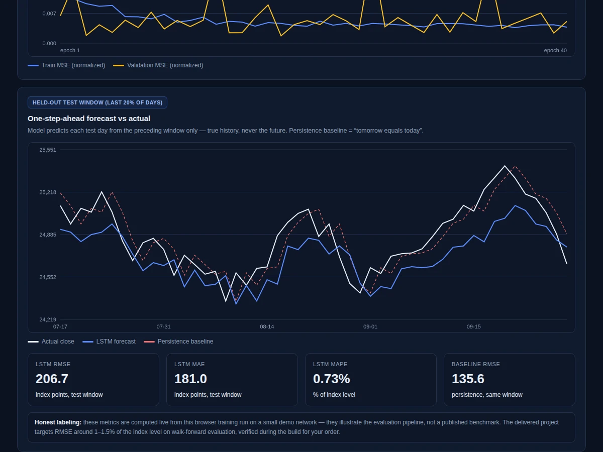
- The web demo embeds the series and trains a smaller pure-JS LSTM live in the browser, plotting training/validation loss and the one-step-ahead forecast against actual closes.
Tech stack:
- Python 3, TensorFlow/Keras
- yfinance (NSE data fetch), pandas, NumPy
- scikit-learn (scaling, metrics)
- Matplotlib (evaluation plots)
- Jupyter Notebook (training & evaluation)
- HTML/CSS/JavaScript (in-browser LSTM demo)
Dataset & model details
- Dataset: NIFTY-50 index (^NSEI) daily OHLCV from the National Stock Exchange of India via Yahoo Finance. Reference build: 249 trading days, 27 Sep 2024 – 26 Sep 2025, 5 feature columns per day (Open, High, Low, Close, Volume).
- Task: Univariate time-series regression — input = 15-day window × 5 features, output = next trading day's closing level in index points.
- Model: Sequence-to-one LSTM: LSTM(32, tanh/sigmoid gates) → Dropout(0.2) → Dense(1, linear); approximately 5,000 parameters; Adam optimizer (lr 0.005), MSE loss, early stopping.
- Metrics: RMSE, MAE and MAPE on chronological held-out folds under walk-forward retraining, reported alongside the persistence baseline. Design target: MAPE around 1% of the index level. No metric is claimed as measured — the build report records the figures achieved by the training run executed for the order.
| Parameter | Value |
|---|---|
| Data window | 249 trading days (reference build; expected) |
| Input shape | 15 days × 5 features per sample (design) |
| Model parameters | Approximately 5,000 (design target) |
| Forecast horizon | 1 trading day ahead (next-day close) |
| Test MAPE | Around 1% of index level (design target, not a measured claim) |
| Training time | Approximately 2–5 min on a laptop CPU (expected) |
| Demo | Single-file web app, trains in-browser, runs offline after download |
| Baseline | Persistence — predict the previous close |
Project features
- [Real NIFTY-50 data pipeline] Daily OHLCV for the NIFTY-50 index (^NSEI) pulled from NSE archives via yfinance into a cleaned, documented CSV — no synthetic or hand-made price series anywhere.
- [Leakage-free sequence preparation] 15-day sliding windows with a strictly chronological 80/20 split; min-max scalers are fit on the training portion only, exactly as a deployed forecaster would require.
- [LSTM forecaster (Keras)] Single-layer LSTM with 32 units, dropout 0.2 and a linear Dense(1) output — roughly 5,000 parameters, trained with Adam on MSE with early stopping.
- [Walk-forward evaluation] Expanding-window retraining with RMSE, MAE and MAPE scored per fold, so performance is measured the way a real forecasting workflow measures it.
- [Persistence baseline] "Tomorrow equals today" runs on the same folds — the honest first bar every price model must clear, and a strong viva talking point when it is hard to beat.
- [In-browser live training demo] A pure-JavaScript LSTM (forward pass, backpropagation through time, Adam, dropout) trains on the embedded real series with live loss curves and a forecast-vs-actual overlay.
- [Price explorer dashboard] Interactive chart of the full series with 20/50-day moving averages, volume overlay and OHLC hover detail.
- [Viva-ready documentation] Report, PPT and Q&A covering LSTM gates, why shuffling time series is wrong, and how to interpret RMSE/MAPE honestly.
What is included
- Python data-fetch and preprocessing scripts (yfinance → cleaned NIFTY-50 CSV)
- Training and walk-forward evaluation Jupyter notebook
- Trained Keras model file with fitted scalers
- Live web demo: price explorer, architecture views, in-browser LSTM training with loss curves and forecast overlay
- Evaluation plots: loss curves, forecast-vs-actual, baseline comparison
- Project report PDF (background, LSTM theory, methodology, honest results discussion)
- PPT presentation for final review
- Viva Q&A preparation document (LSTM gates, leakage, baselines, metric interpretation)
Limitations & prerequisites
- Daily index prices behave close to a random walk — a well-tuned LSTM may not beat the persistence baseline on every fold; the report shows both numbers honestly.
- Single-day horizon only: the model predicts the next close, not multi-day trajectories, which compound error quickly.
- Fitted on one index and one market regime — elections, crashes or policy shocks degrade any model trained on calm-period data.
- The ~1% MAPE figure is a design target, never a measured claim; the achieved metrics are recorded after the build run for your order.
- yfinance/NSE data revisions or missing sessions must be re-validated on each fresh data pull; the pipeline documents the check.
- This is a forecasting study, not a trading system: no backtester, no transaction costs, no position sizing — nothing here implies profitability.
Frequently Asked Questions
Which dataset is used and is it real?
Yes, real. Daily open-high-low-close-volume for the NIFTY-50 index (^NSEI) from the National Stock Exchange via Yahoo Finance — 249 trading days in the reference build. The demo embeds this exact series, so every chart you see is genuine market data, not generated.
Why an LSTM instead of a simpler model?
Prices carry short-term memory — trend, weekly rhythm, volatility clustering — that feed-forward models ignore. The LSTM's gating lets it keep or discard information across the 15-day window. The project still benchmarks against persistence, so the LSTM has to earn its complexity rather than assume it.
What does the live web demo actually train?
A genuine LSTM written in pure JavaScript — forward pass, backpropagation through time, Adam, dropout — training on the embedded real NIFTY-50 series with a fixed seed. It plots train/validation loss live, then overlays its one-step-ahead forecasts against actual closes with RMSE, MAE and MAPE.
Can this be used to make money trading?
No, and the project states that plainly. Forecasting error of ~1% of the index level is large next to typical daily moves, and the build includes no backtester, costs or risk controls. It is a rigorous ML study of time-series forecasting, suitable for academic evaluation.
What if the model does not beat the persistence baseline?
That is a legitimate, reportable result — daily index data is notoriously close to a random walk. The report documents both sets of metrics and the Q&A prepares you to discuss exactly why beating "tomorrow equals today" is hard, which examiners respect more than an inflated claim.
Is this project suitable for a final-year project?
Yes — for AI & Machine Learning, Computer Science and IT programs. It demonstrates time-series methodology done properly: leakage-free data preparation, LSTM architecture design, walk-forward evaluation, and honest baseline comparison against persistence. The live in-browser training demo gives examiners something concrete to interact with, and the Q&A document prepares answers for the hard questions on gates, metrics and market efficiency. Suitable for B.E./B.Tech final-year projects in AI & Machine Learning, Computer Science and IT.
Components & software requirements
- Python 3, TensorFlow/Keras
- yfinance (NSE data fetch), pandas, NumPy
- scikit-learn (scaling, metrics)
- Matplotlib (evaluation plots)
- Jupyter Notebook (training & evaluation)
- HTML/CSS/JavaScript (in-browser LSTM demo)
Dataset & model details
- Dataset: NIFTY-50 index (^NSEI) daily OHLCV from the National Stock Exchange of India via Yahoo Finance. Reference build: 249 trading days, 27 Sep 2024 – 26 Sep 2025, 5 feature columns per day (Open, High, Low, Close, Volume).
- Task: Univariate time-series regression — input = 15-day window × 5 features, output = next trading day's closing level in index points.
- Model: Sequence-to-one LSTM: LSTM(32, tanh/sigmoid gates) → Dropout(0.2) → Dense(1, linear); approximately 5,000 parameters; Adam optimizer (lr 0.005), MSE loss, early stopping.
- Metrics: RMSE, MAE and MAPE on chronological held-out folds under walk-forward retraining, reported alongside the persistence baseline. Design target: MAPE around 1% of the index level. No metric is claimed as measured — the build report records the figures achieved by the training run executed for the order.
Delivery information
Built-to-order project. Delivery timeline is shared after order confirmation based on current queue.
Support terms
Complete documentation, setup guide, and viva preparation included. Support for setup and explanation provided.