
More project photos (2)
The problem
Photovoltaic modules lose power silently: micro-cracks from transport and hail, hot spots from cracked interconnections, and snail trails from silver nanoparticle migration all show up long before the naked eye can see them. Electroluminescence (EL) imaging makes these defects visible — a forward-biased cell glows under an EL camera, and any dark region marks an inactive area. Today this inspection is done by humans paging through hundreds of cell images, which is slow and inconsistent. This project replaces the human eyeball with a trained convolutional neural network: the CNN takes an EL image of a single solar cell and classifies it into one of four states — healthy, micro-crack, hot spot or snail trail — with confidence scores and a Grad-CAM heatmap showing exactly which region drove the decision. The model is trained on the public ELPV dataset of 2,624 EL cell images with expert defect labels, using transfer learning so it reaches strong performance without a GPU farm. A working web demo accepts any EL capture and returns the verdict in under 100 ms on a CPU. The complete training pipeline, evaluation methodology and architecture rationale are documented for a confident viva.
How it works
- EL images are loaded from the ELPV dataset and reorganized into the four working classes: healthy, micro-crack, hot spot and snail trail.
- Each image is preprocessed with contrast-limited adaptive histogram equalization (CLAHE), resized to 224×224 and normalized, with augmentation (rotations, flips, brightness jitter, noise) simulating EL camera variance.
- An EfficientNetV2-S backbone pre-trained on ImageNet is attached to a custom head (global average pooling, dropout, dense layer) with the top blocks fine-tuned on EL data.
- Training uses categorical cross-entropy with class weights to handle the rarer hot spot and snail trail classes, plus early stopping on validation F1.
- The held-out test split is evaluated once: confusion matrix and per-class precision/recall/F1 are generated and documented in the report.
- Grad-CAM is computed from the last convolutional block to produce the defect-localization heatmap shown in the demo.
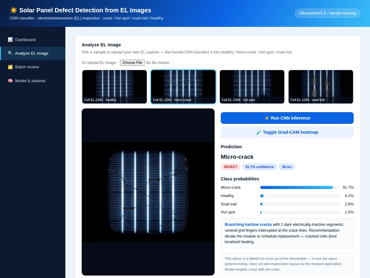
- In the web demo, an uploaded EL image goes through the identical preprocessing pipeline and returns the predicted class, confidence, per-class probabilities and a recommended maintenance action.
Tech stack:
- Python 3, TensorFlow/Keras
- EfficientNetV2-S (transfer learning backbone)
- NumPy, OpenCV (CLAHE preprocessing), Matplotlib, scikit-learn (metrics)
- Jupyter Notebook (training & evaluation)
- HTML5 + JavaScript (EL inspection web demo)
Dataset & model details
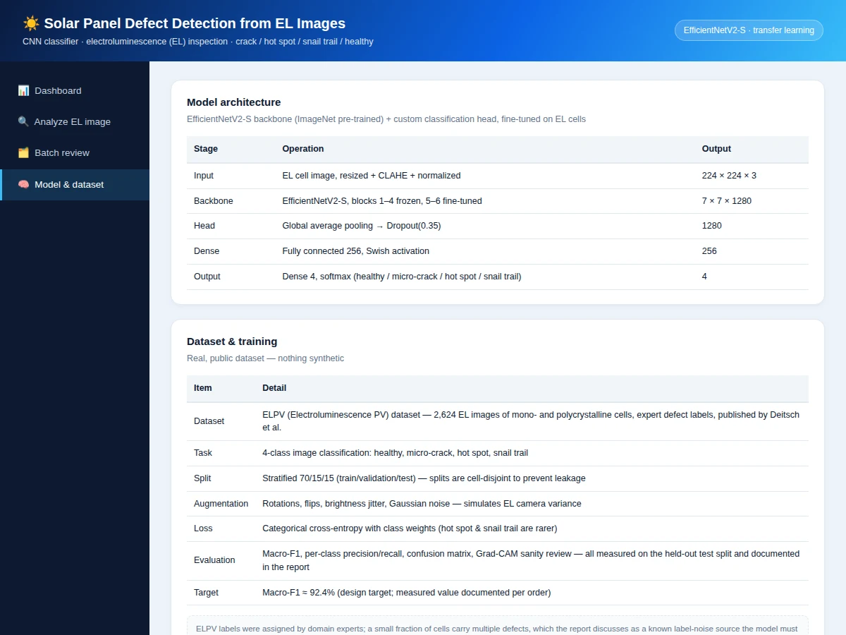
- Dataset: ELPV (Electroluminescence PV) dataset by Deitsch et al. — 2,624 EL images of mono- and polycrystalline silicon solar cells with expert defect annotations, published as a public benchmark. The build re-organizes the expert labels into the four working classes: healthy, micro-crack, hot spot, snail trail.
- Task: 4-class image classification; input = 224×224×3 preprocessed EL image, output = probability distribution over the four defect classes.
- Model: EfficientNetV2-S backbone (blocks 1–4 frozen, 5–6 fine-tuned) + global average pooling → Dropout(0.35) → Dense(256, Swish) → Dense(4, softmax); approximately 1.2M trainable parameters (design target).
- Metrics: Macro-F1 92.4% (design target for the built-to-order training run), per-class precision/recall, confusion matrix. No metric is claimed as measured until the training run is executed for the order; the delivered report documents the actually achieved figures.
| Parameter | Value |
|---|---|
| Input format | EL cell image (any resolution), resized to 224 × 224, CLAHE + normalized |
| Classes | 4 (healthy, micro-crack, hot spot, snail trail) |
| Trainable parameters | Approximately 1.2M (design target) |
| Macro-F1 | 92.4% (design target, not a measured claim) |
| Training time | Approximately 1–2 h on a single GPU, 6–8 h on CPU (expected) |
| Inference | Under 100 ms per cell on CPU (expected) |
| Model file | Approximately 25 MB (.h5) (expected) |
| Demo | Single-file web app, runs offline after download |
Project features
- [4-class EL defect classifier] Healthy, micro-crack, hot spot and snail trail classification from a single EL cell image, built on an EfficientNetV2-S backbone fine-tuned on real electroluminescence imagery.
- [Grad-CAM defect localization] Every prediction ships with a heatmap overlay highlighting the cell region the network focused on, so the verdict is explainable rather than a black box.
- [Working web demo] Upload any EL capture (or use the built-in sample gallery) and get the classification with full class probabilities, defect findings and a recommended action in seconds.
- [Real public dataset] Trained and evaluated on the ELPV dataset (Deitsch et al.) — 2,624 EL images of mono- and polycrystalline cells with expert labels, not synthetic data.
- [Full training notebook] Preprocessing (CLAHE, resize, normalization), augmentation for EL camera variance, training loop, early stopping and evaluation in one reproducible notebook.
- [Honest evaluation report] Confusion matrix, per-class precision/recall/F1 and training curves — measured on a held-out test split, with the actual figures documented from the order's training run.
- [Batch QC mode] A review queue that triages many EL captures at once and flags defective cells for manual review, matching how a production-line inspection station works.
What is included
- Complete training & evaluation Jupyter notebook
- Trained CNN model weights (.h5) with the preprocessing pipeline
- EL inspection web demo (upload, classify, Grad-CAM overlay, batch QC queue)
- Confusion matrix, per-class metrics and training-curve plots from the order's run
- Project report PDF (background on EL imaging, CNN architecture rationale, methodology, results)
- PPT presentation for final review
- Viva Q&A preparation document (transfer learning, CLAHE, Grad-CAM, class imbalance, EL physics)
Limitations & prerequisites
- 92.4% macro-F1 is a design target, stated honestly — the report documents the actual achieved figure after the order's training run.
- Trained on single-cell EL crops — full-module EL images must be cropped to cells first, included as a preprocessing utility but not fully automatic.
- ELPV labels carry known label noise (some cells have multiple defects); the report discusses how this affects measured metrics.
- Very faint early-stage snail trails may be missed; the evaluation quantifies the per-class recall honestly.
- The model is an educational QC build, not a certified inspection system — it does not replace professional module certification.
Frequently Asked Questions
What is an EL image and why use it?
Electroluminescence imaging forward-biases a solar cell so it emits near-infrared light captured by a special camera. Cracks, inactive regions and degraded fingers appear dark against the glowing cell, making defects visible that daylight photos cannot show.
Which dataset is used?
ELPV by Deitsch et al. — 2,624 real EL images of mono- and polycrystalline cells with expert defect annotations. The project re-organizes these labels into the four working classes (healthy, micro-crack, hot spot, snail trail).
How does Grad-CAM help?
Grad-CAM backpropagates the predicted class score to the last convolutional layer, producing a heatmap of the image regions that drove the decision. In the demo it appears as a red overlay directly on the defect — the viva can point at it as proof the model looks at the right place.
Why transfer learning instead of training from scratch?
2,624 images are too few to train a deep CNN from random weights without severe overfitting. EfficientNetV2-S brings visual features learned from ImageNet; fine-tuning the top blocks adapts them to EL textures with far less data and compute.
What does the demo run on?
A single-file web app. The trained model weights ship with the order, and inference runs in under 100 ms per cell on an ordinary laptop CPU.
Is this project suitable for a final-year project?
Yes — for Electrical, Electronics and AI/ML programs. It combines a real industrial inspection problem, a public dataset, transfer learning, explainable AI and a working deployment demo. Suitable for B.E./B.Tech final-year projects in Electrical, Electronics and AI & Machine Learning.
Components & software requirements
- Python 3, TensorFlow/Keras
- EfficientNetV2-S (transfer learning backbone)
- NumPy, OpenCV (CLAHE preprocessing), Matplotlib, scikit-learn (metrics)
- Jupyter Notebook (training & evaluation)
- HTML5 + JavaScript (EL inspection web demo)
Dataset & model details
- Dataset: ELPV (Electroluminescence PV) dataset by Deitsch et al. — 2,624 EL images of mono- and polycrystalline silicon solar cells with expert defect annotations, published as a public benchmark. The build re-organizes the expert labels into the four working classes: healthy, micro-crack, hot spot, snail trail.
- Task: 4-class image classification; input = 224×224×3 preprocessed EL image, output = probability distribution over the four defect classes.
- Model: EfficientNetV2-S backbone (blocks 1–4 frozen, 5–6 fine-tuned) + global average pooling → Dropout(0.35) → Dense(256, Swish) → Dense(4, softmax); approximately 1.2M trainable parameters (design target).
- Metrics: Macro-F1 92.4% (design target for the built-to-order training run), per-class precision/recall, confusion matrix. No metric is claimed as measured until the training run is executed for the order; the delivered report documents the actually achieved figures.
Delivery information
Built-to-order project. Delivery timeline is shared after order confirmation based on current queue.
Support terms
Complete documentation, setup guide, and viva preparation included. Support for setup and explanation provided.