
More project photos (2)
The problem
Every retailer lives or dies on one question: how much of each product will sell next week. Order too much and cash sits on shelves expiring; order too little and shelves go empty, customers leave, and the sale is lost forever. Human buyers forecast by gut feel and spreadsheets, which breaks down across thousands of SKUs with seasonal spikes and festivals interacting at once. The data to do better already exists — every point-of-sale system logs what sold, when, and at what price. The challenge is turning that history into future numbers without leaking the future into the training data, which is the time-series trap. This project builds that pipeline: feature engineering over lags and calendar effects, three models (ARIMA, Prophet, XGBoost) compared on walk-forward splits, and forecasts converted into inventory decisions — reorder points and safety stock — the way a retail planning team would use them.
How it works
- Historical sales data (CSV) is uploaded — date, SKU, units sold, price, promo flags, holidays.
- Feature engineering builds lag features, rolling statistics, calendar features and promo/holiday indicators.
- The data is split with walk-forward validation: models train on the past and are tested on genuinely future windows.
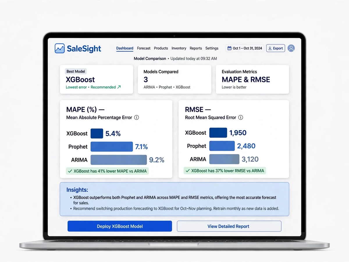
- ARIMA, Prophet and XGBoost are trained; MAPE and RMSE are computed per model and per SKU.
- The best model (typically XGBoost) generates forecasts for the chosen horizon with confidence bands.
- Inventory logic converts forecasts into reorder points, safety stock and days-of-cover recommendations.
- The SaleSight dashboard visualizes everything and exports forecasts to CSV.
Project features
- Multi-model forecasting: XGBoost, Prophet and ARIMA on the same dataset, side by side
- Time-series feature engineering: lags, rolling means, day-of-week, month, holiday flags, promo indicators
- Per-SKU and category-level forecasts with configurable horizon (7/30/90 days)
- Forecast-vs-actual interactive charts with confidence intervals
- Model comparison view: MAPE and RMSE bars for ARIMA, Prophet and XGBoost
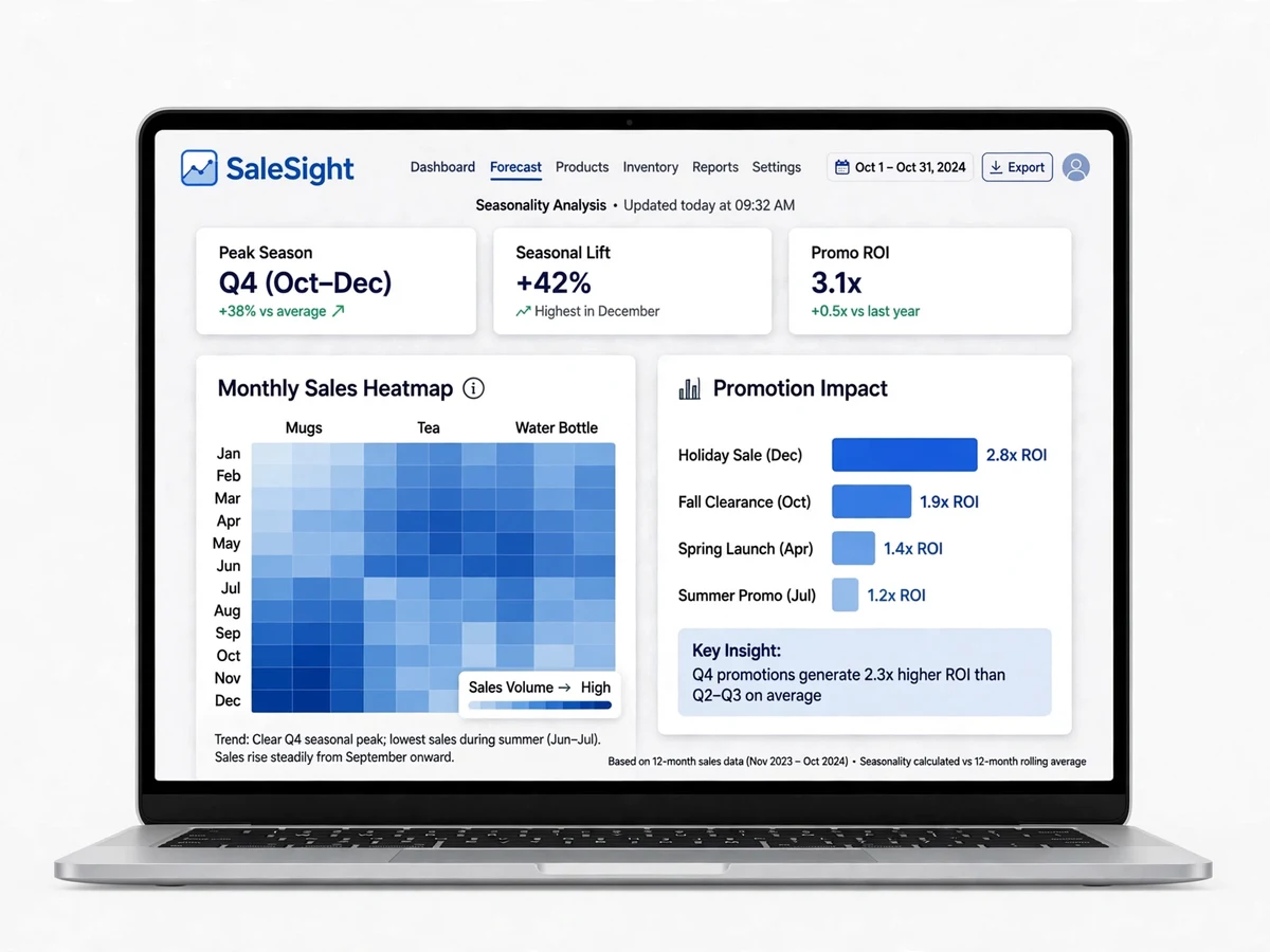
- Seasonality analysis: monthly heatmap, weekday patterns, promotion-lift charts
- Inventory recommendations: reorder point, safety stock and days-of-cover per SKU
- What-if simulator: adjust promo intensity or price and see the forecast respond
- SaleSight Streamlit dashboard: upload CSV, train, forecast, export results
- Walk-forward (time-based) validation so no future data leaks into training
What is included
- Complete, commented Python source code (features, training, evaluation, dashboard)
- Trained models for the sample dataset, ready to forecast immediately
- SaleSight Streamlit dashboard application
- Project report PDF (literature survey, feature design, walk-forward methodology, model comparison tables)
- PPT presentation
- Viva Q&A document (time-series leakage, MAPE vs RMSE, XGBoost vs ARIMA, seasonality)
- Setup guide (environment, dependencies, sample dataset format)
FAQs
- Why is sales forecasting a good machine-learning topic? It compares classical time-series (ARIMA, Prophet) against gradient boosting (XGBoost) with proper walk-forward validation — no future data leaking into training — and the forecasts feed real decisions: reorder points and safety stock.
- How are the models compared? All three train on the same features and walk-forward splits; the dashboard shows MAPE and RMSE bars per model and per SKU, so the choice of XGBoost is defended with numbers, not asserted.
- What data is needed? Any CSV with date, product/SKU, units sold — plus optional price, promotion and holiday columns. A retail-style sample dataset is included so it runs out of the box.
- Is a GPU needed? No — XGBoost on tens of thousands of rows trains in seconds on a CPU; the whole pipeline runs on a standard laptop.
- Can it be demoed live? Yes — upload the sample data or your own CSV, pick a horizon, and the dashboard shows forecast-vs-actual charts, model comparison and inventory recommendations.
- What are the natural extensions? Hierarchical forecasting (SKU to category to store), deep models like LSTM or Temporal Fusion Transformer, or a live inventory-alert system tied to the reorder points.
Limitations & prerequisites
- Forecasts are only as good as the history: new SKUs with no sales history get weak cold-start predictions.
- Sudden demand shocks (viral trends, supply disruptions) cannot be predicted from historical patterns.
- MAPE blows up on near-zero sales days; the report explains this and reports RMSE alongside.
- External drivers (competitor pricing, weather, marketing spend) are not modelled unless provided as features.
Components & software requirements
- Python 3.9+ (Pandas, NumPy, scikit-learn)
- XGBoost (gradient-boosted demand model)
- Prophet / statsmodels ARIMA (classical time-series baselines)
- Streamlit (SaleSight forecasting dashboard)
- Matplotlib/Plotly (forecast charts, heatmaps, comparison bars)
Specifications
| Parameter | Value |
|---|---|
| Models | XGBoost (primary), Prophet, ARIMA (baselines) |
| Features | Lags (7/14/28d), rolling means, calendar, holidays, promo flags, price |
| Forecast horizon | 7, 30 or 90 days; per SKU and per category |
| Validation | Walk-forward (expanding-window) time-series split — no leakage |
| Key metrics | MAPE, RMSE per model; XGBoost typically 8–15% MAPE on retail-style data |
| Seasonality | Monthly heatmap, weekday profile, promo-lift analysis |
| Inventory outputs | Reorder point, safety stock, days of cover per SKU |
| What-if | Promo intensity and price sliders re-run the forecast live |
| Dashboard | Streamlit; CSV upload, training, comparison, export |
| Sample data | Included retail-style dataset; works with your own CSV in the same format |