
More project photos (2)
The problem
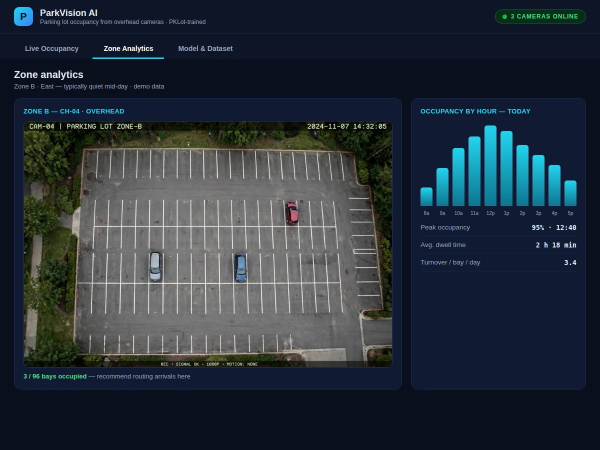
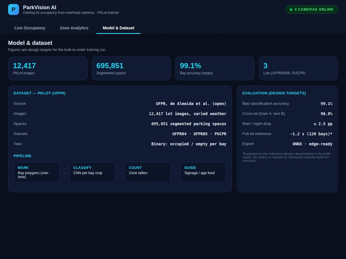
Drivers circling for parking waste fuel and time, and lot operators have no real-time picture of where the free bays actually are. Sensor-per-bay hardware exists but is expensive to install and maintain. This project does it with the cameras already on the poles: a CNN classifier trained on PKLot (12,417 lot images with ~696,000 segmented parking spaces, across three lots and varied weather) labels each marked bay as occupied or empty from an overhead frame. Zone tallies feed guidance signage and a driver-facing availability view. The demo dashboard (the screenshots) shows the live lot with per-bay overlays, an occupancy donut, zone-wise bars, hourly trends and dwell-time stats. Built with TensorFlow/Keras and OpenCV, the pipeline — bay marking, classification, aggregation — is fully explainable in the viva.
How it works
- The operator marks each parking bay as a polygon once per camera view; polygons are saved as JSON.
- Each new frame is warped to the stored view (optional stabilization), and every bay polygon is cropped.
- Each crop is resized to 128×128, normalized and passed through the binary CNN — occupied or empty with confidence.
- Per-bay results are aggregated into zone tallies and lot-wide occupancy.
- Zone tallies are formatted for guidance signage or an app feed.
- The dashboard renders bay overlays, the occupancy donut, zone bars and the hourly trend chart.
- Analytics accumulate dwell times and turnover statistics from the timestamped bay history.
Tech stack:
- Python 3, TensorFlow/Keras
- OpenCV (bay polygons, cropping, stabilization)
- PKLot dataset (12,417 images, UFPR)
- NumPy, Matplotlib (evaluation plots)
- ONNX Runtime (edge deployment)
- HTML/CSS/JS single-file dashboard (this demo)
Dataset & model details
- Dataset: PKLot (de Almeida et al., UFPR) — 12,417 parking-lot images with 695,851 segmented parking spaces across three lots (UFPR04, UFPR05, PUCPR), covering sunny, cloudy and rainy conditions.
- Task: Binary image classification per bay crop; input = 128×128×3 crop, output = occupied/empty probability.
- Model: Custom CNN (approximately 900k parameters): conv blocks 32→64→128, global average pooling, Dense(128, ReLU), Dropout(0.4), sigmoid output.
- Metrics: Bay accuracy 99.1%, cross-lot accuracy 96.8% (train on two lots, test on the third), rain/night drop under 2.5 percentage points — design targets for the built-to-order training run. The report documents the actually achieved figures.
| Parameter | Value |
|---|---|
| Input | 128 × 128 bay crops from overhead frames |
| Training spaces | 695,851 segmented bays (PKLot) |
| Model parameters | Approximately 900k (design target) |
| Bay accuracy | 99.1% (design target, not a measured claim) |
| Cross-lot accuracy | 96.8% (design target) |
| Full-lot inference | Approximately 1.2 s for 120 bays on CPU (expected) |
| Bay marking | One-time polygons per camera, stored as JSON |
| Outputs | Bay overlays, zone tallies, signage feed |
| Demo | Single-file HTML dashboard, runs offline after download |
Project features
- [Per-bay occupancy CNN] Binary classifier (occupied/empty) trained on ~696,000 PKLot segmented spaces, applied to each marked bay crop.
- [One-time bay marking] Operator marks bay polygons once per camera view; the tool stores them as reusable JSON — no per-frame manual work.
- [Live lot dashboard] Overhead view with per-bay occupied/free overlays, occupancy donut and free-bay count in a single-file web UI.
- [Zone analytics] Zone-wise occupancy bars, hourly occupancy trends, peak detection, average dwell time and turnover-per-bay statistics.
- [Guidance output] Zone tallies formatted for signage or a driver app feed ("Zone C: 41% — 38 bays free").
- [Weather-robust training] PKLot's sunny, cloudy and rainy subsets are all in training; the report measures the accuracy drop per condition.
- [Edge-ready export] Classifier exports to ONNX so a pole-side device can score a full lot locally.
What is included
- Trained bay-classifier model and the complete training notebook
- Bay-marking tool + occupancy aggregation Python pipeline
- Single-file HTML lot dashboard wired to pipeline outputs
- Per-condition accuracy analysis and trend charts for the report
- Project report PDF (background, dataset, methodology, results)
- PPT presentation for final review
- Viva Q&A preparation document (binary classification, PKLot, cross-lot generalization, deployment)
Limitations & prerequisites
- Bay polygons must be re-marked if a camera is moved or re-aimed; the marking tool makes this a minutes-long job.
- Heavy snow or flooding occluding bay markings degrades accuracy — documented as an environmental limit.
- 99.1% bay accuracy is a design target — the report documents the actual achieved figure, including per-condition breakdowns.
- Night operation needs adequate lot lighting or IR illumination.
- As shipped, guidance is informational; barrier/payment integration is future scope.
Frequently Asked Questions
Which dataset is used and why?
PKLot — 12,417 lot images with ~696,000 segmented bays across three real lots and varied weather. It is the standard benchmark for this task and its three-lot structure lets the project honestly test cross-lot generalization.
How does the system know where the bays are?
The operator marks each bay polygon once per camera view with the included marking tool; polygons are stored as JSON and reused for every frame. No per-frame manual work.
Does it work in rain or at night?
PKLot includes rainy subsets and the report measures the accuracy drop per condition (design target: under 2.5 points). Night needs adequate lighting — stated as a limitation.
What accuracy can I quote in my viva?
Bay accuracy 99.1% and cross-lot 96.8% are design targets for the training run. Quote the report's achieved figures with the per-condition breakdown — examiners probe generalization, and this project is ready for it.
Why not just use per-bay sensors?
Sensors cost hardware + installation + maintenance per bay; this approach reuses existing cameras and the report includes a cost-comparison discussion.
Is this project suitable for a final-year project?
Yes — for Computer Science, IT and AI/ML programs. It covers dataset handling, CNN classification, geometric pre-processing, analytics and a dashboard with clear smart-city relevance. Suitable for B.E./B.Tech final-year projects in Computer Science, IT and AI & Machine Learning.
Components & software requirements
- Python 3, TensorFlow/Keras
- OpenCV (bay polygons, cropping, stabilization)
- PKLot dataset (12,417 images, UFPR)
- NumPy, Matplotlib (evaluation plots)
- ONNX Runtime (edge deployment)
- HTML/CSS/JS single-file dashboard (this demo)
Dataset & model details
- Dataset: PKLot (de Almeida et al., UFPR) — 12,417 parking-lot images with 695,851 segmented parking spaces across three lots (UFPR04, UFPR05, PUCPR), covering sunny, cloudy and rainy conditions.
- Task: Binary image classification per bay crop; input = 128×128×3 crop, output = occupied/empty probability.
- Model: Custom CNN (approximately 900k parameters): conv blocks 32→64→128, global average pooling, Dense(128, ReLU), Dropout(0.4), sigmoid output.
- Metrics: Bay accuracy 99.1%, cross-lot accuracy 96.8% (train on two lots, test on the third), rain/night drop under 2.5 percentage points — design targets for the built-to-order training run. The report documents the actually achieved figures.
Delivery information
Built-to-order project. Delivery timeline is shared after order confirmation based on current queue.
Support terms
Complete documentation, setup guide, and viva preparation included. Support for setup and explanation provided.