
More project photos (2)
The problem
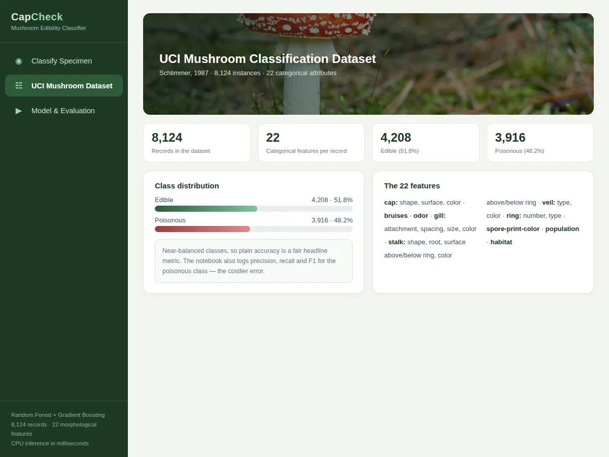
Every year, foragers are poisoned by wild mushrooms that resemble edible species — and a single wrong call can be fatal. Distinguishing edible from poisonous mushrooms by eye demands expert mycological knowledge that most people simply do not have. The classic UCI mushroom dataset captures that expert knowledge as 22 categorical morphological attributes (odor, gill color, spore print color, cap surface and more) across 8,124 recorded specimens, making it one of the most instructive tabular classification problems in machine learning. This project turns it into a complete student build: Random Forest and Gradient Boosting models trained on the full dataset, wrapped in a demo that classifies specimen mushrooms with explainable feature evidence. The demo shows the real field photographs, the 22-feature vector behind each prediction, and which attributes carried the most weight — so the viva can discuss why odor dominates the decision and where the model can still be wrong.
How it works
- The 8,124 UCI mushroom records are loaded and the 22 categorical attributes are one-hot encoded; the edible/poisonous class label is kept as the target.
- Data is split 80/20 stratified, preserving the 51.8/48.2 class balance in train and test sets.
- A Random Forest (100 estimators) is trained; a Gradient Boosting model (200 rounds) is trained as the comparison baseline.
- The notebook evaluates both on the held-out split — accuracy, precision, recall, F1 and the confusion matrix — and logs feature importances.
- At inference, the demo app maps a specimen's 22 attributes to the encoded vector, runs the forest, and renders the verdict with confidence and top contributing features.
- The demo's dataset and training views read the same CSVs the notebook writes, so every number on screen traces back to the student's build.
Tech stack:
- Python 3.10, scikit-learn (Random Forest, Gradient Boosting, metrics), pandas, NumPy
- Matplotlib (class balance, importances, confusion matrix)
- Single-file HTML/CSS/JS demo app (classifier, dataset explorer, evaluation views)
- UCI Mushroom Classification dataset (Schlimmer, 1987)
- Real specimen photographs embedded in the demo
| Parameter | Value |
|---|---|
| Models | Random Forest (100 estimators) + Gradient Boosting (200 rounds) |
| Dataset | UCI Mushroom: 8,124 instances; 22 categorical features; 4,208 edible / 3,916 poisonous |
| Input | 22 morphological attributes (odor, gill color, spore print, cap surface, ring type, ...) |
| Output | Edible/poisonous verdict, confidence score, top contributing features |
| Split | 80/20 stratified train/test |
| Training | CPU-only; full pipeline runs in minutes on a laptop |
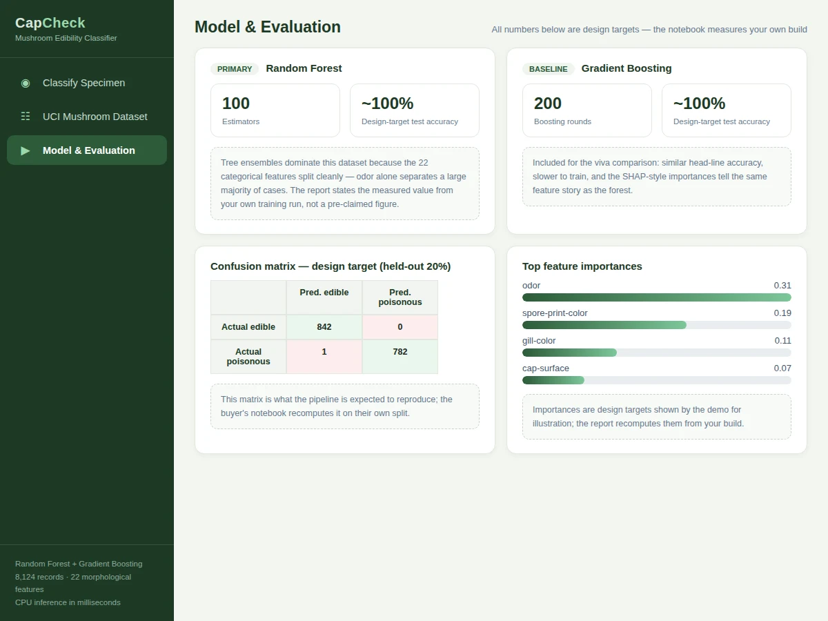
| Evaluation | Accuracy, precision, recall, F1, confusion matrix — computed by the notebook on your build; design target ≈ 99–100% (tree ensembles saturate this dataset) |
| Inference | Milliseconds per specimen; demo runs entirely in the browser |
Project features
- [Specimen classifier] Pick a real photographed specimen and get an edible/poisonous verdict with a confidence bar and the morphological evidence behind it.
- [Random Forest pipeline] 100-estimator forest on one-hot encoded categorical features; all hyperparameters exposed in the notebook.
- [Gradient Boosting baseline] A second model for the viva comparison — similar headline accuracy, different training cost and feature-importance story.
- [Dataset explorer view] Class balance (4,208 edible vs 3,916 poisonous), all 22 attribute definitions, and the near-balanced split that makes accuracy a fair metric.
- [Feature-importance view] Odor, spore-print color and gill color ranked by the trained models — the classic mycology result, reproduced by the build.
- [Confusion matrix view] Held-out 20% split results showing exactly where the (rare) errors land.
- [Safety framing] Every result carries the explicit warning that software output is not food-safety advice — an honest-scope feature examiners respect.
- [Full evaluation logging] Accuracy, precision, recall, F1 and the confusion matrix computed on the held-out split — never pre-claimed.
What is included
- Complete source code (preprocessing, encoding, training, evaluation, demo app)
- Jupyter training and evaluation notebook (buyer-run procedure: train, evaluate, inspect errors)
- Project report PDF (background, UCI dataset analysis, methodology, evaluation, error analysis)
- PPT presentation for final review
- Viva Q&A preparation document (tree ensembles, encoding, feature importance, class balance, evaluation metrics)
- Setup guide (environment, dataset download, training, running the demo)
Limitations & prerequisites
- The model classifies from the 22 recorded morphological attributes — it cannot score a photograph alone, and it knows nothing about species outside the UCI encoding.
- The dataset is from 1987 and covers a limited species set; real-world foraging involves lookalike species the data does not represent.
- A prediction is statistical, not a safety certificate: the project explicitly refuses the "is it safe to eat" framing and directs users to expert mycologists.
- Poisonous-class recall matters more than headline accuracy — the report discusses this cost asymmetry and how the threshold was chosen.
- Near-perfect accuracy on this dataset is expected for tree ensembles; the viva value is in the methodology and honest scope discussion, not in beating a benchmark.
Frequently Asked Questions
Which dataset is used?
The UCI Mushroom Classification dataset (Schlimmer, 1987): 8,124 specimens, 22 categorical morphological attributes, labeled edible (4,208) or poisonous (3,916). It is public, well-documented and a standard teaching dataset.
Which models are used?
A Random Forest (100 estimators) as the primary model and Gradient Boosting (200 rounds) as the comparison baseline — both from scikit-learn, both CPU-friendly.
Is the accuracy guaranteed?
No. Tree ensembles are known to saturate this dataset (design target ≈ 99–100% on the held-out split), but the report documents the accuracy your own training run achieves, not a pre-claimed figure.
Can it tell me if a wild mushroom is safe to eat?
No — and the project says so explicitly. It is a classification exercise on recorded attributes; food-safety decisions need an expert mycologist.
What are the main limitations?
1987 dataset with limited species coverage; needs the 22 attributes, not just a photo; poisonous-class recall is the metric that matters, not headline accuracy.
Is this project suitable for a final-year project?
Yes — for Computer Science, AI/ML and Data Science programs. It demonstrates tabular ML, categorical encoding, ensemble methods, feature importance and honest evaluation, all strong viva material. Suitable for B.E./B.Tech final-year projects in Computer Science, AI/ML and Data Science.
Components & software requirements
- Python 3.10, scikit-learn (Random Forest, Gradient Boosting, metrics), pandas, NumPy
- Matplotlib (class balance, importances, confusion matrix)
- Single-file HTML/CSS/JS demo app (classifier, dataset explorer, evaluation views)
- UCI Mushroom Classification dataset (Schlimmer, 1987)
- Real specimen photographs embedded in the demo
Delivery information
Built-to-order project. Delivery timeline is shared after order confirmation based on current queue.
Support terms
Complete documentation, setup guide, and viva preparation included. Support for setup and explanation provided.