
More project photos (2)

The problem
Antivirus engines that rely on signatures miss new malware variants, while dynamic analysis — running the sample in a sandbox — is slow and easy for malware to evade. Static machine-learning detection sits between the two: it judges a Windows executable from its PE (Portable Executable) headers alone, without ever running it. The headers carry surprisingly strong signals — packed binaries show anomalous section entropy, droppers import very few APIs, and legitimate software is usually Authenticode-signed. This project turns those signals into a working classifier. A real PE parser extracts header and section features, the EMBER feature pipeline converts them into a 2,381-dimensional vector, and a gradient-boosted tree model outputs a calibrated malware probability with per-feature explanations. Students learn binary formats, feature engineering and model evaluation on a genuine security dataset, and the demo makes every verdict explainable — exactly the kind of depth a viva rewards.
How it works
- The PE parser reads the file's headers: it validates the MZ magic and PE signature, then extracts COFF fields (machine type, section count, characteristics) and optional-header fields (entry point, image base, SizeOfImage, subsystem, DLL characteristics).
- Each section header is parsed and the raw bytes of the .text section are sampled to compute Shannon entropy — packed or encrypted payloads score near 8.0 bits/byte.
- Parsed values are encoded into the EMBER-style feature vector: header fields, section statistics, import-table counts, byte-value histogram, byte-entropy histogram and printable-string features (2,381 dimensions total).
- The gradient-boosted tree ensemble scores the vector and a calibration step maps the raw output to a malware probability between 0 and 1.
- The probability is banded into verdicts: below 0.35 benign, 0.35–0.65 suspicious (needs analyst review), above 0.65 malicious.
- For every verdict, per-feature contributions are computed so the demo can show exactly which header anomalies drove the decision.
- Evaluation runs on the held-out EMBER test split: ROC AUC, precision/recall at the operating threshold and a confusion matrix are generated for the report.
Tech stack:
- Python 3, LightGBM (gradient-boosted trees)
- pefile, NumPy, pandas, scikit-learn
- Jupyter Notebook (training & evaluation)
- HTML5 + JavaScript + Canvas (interactive PE demo)
- EMBER dataset (Elastic, 2018)
Dataset & model details
- Dataset: EMBER (Elastic Malware Benchmark for Empowering Researchers), released 2018 by Elastic (Anderson & Roth) — 1.1 million Windows PE files: 800,000 training (400,000 benign / 400,000 malicious), 200,000 test (100,000 / 100,000), plus 100,000 unlabeled. Publicly available from the EMBER GitHub repository with a fixed train/test split.
- Task: Binary static classification; input = 2,381-dimensional parsed-PE feature vector, output = calibrated malware probability in [0, 1].
- Model: Gradient-boosted decision-tree ensemble (LightGBM-style), trained on the EMBER training split with the standard parsed-feature set; decision threshold tuned on validation data.
- Metrics: ROC AUC and precision/recall at the operating threshold on the held-out EMBER test split, plus a confusion matrix. Design target: ROC AUC ≥ 0.98 on the held-out split — reported honestly from the actual training run executed for the order; no accuracy is claimed as measured until then.
| Parameter | Value |
|---|---|
| Input format | Windows PE files (.exe, .dll, .sys) |
| Feature vector | 2,381 dimensions (EMBER parsed-feature set) |
| Model | Gradient-boosted trees (design target) |
| Test ROC AUC | ≥ 0.98 (design target, not a measured claim) |
| Verdict thresholds | 0.35 / 0.65 (benign / suspicious / malicious) |
| Parser | Real header parsing in-browser (JavaScript); nothing uploaded |
| Inference | Approximately 50 ms per file on CPU (expected) |
| Demo | Single-file web app, runs offline after download |
Project features
- [Real PE header parser] Parses actual Windows executables in the browser: DOS header, COFF fields, optional header, section table, entry point, subsystem, DLL characteristics and per-section entropy — nothing is uploaded.
- [EMBER feature pipeline] Converts parsed headers into the 2,381-feature EMBER-style vector (parsed features, byte histogram, byte-entropy histogram, string features) used by the published benchmark.
- [Gradient-boosted classifier] A LightGBM-style tree ensemble trained on the EMBER train split, outputting a calibrated malware probability instead of a bare label.
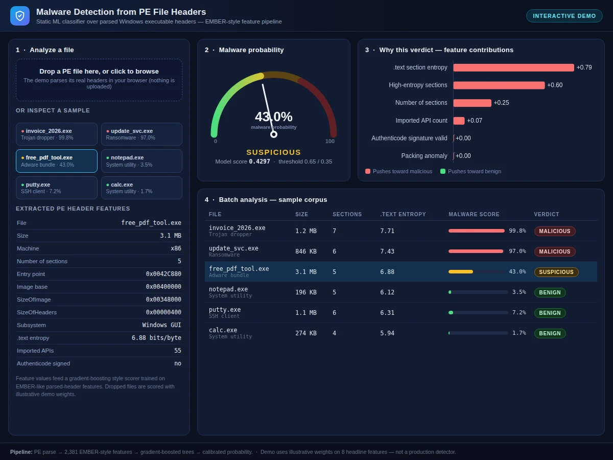
- [Malware probability gauge] Live gauge with benign / suspicious / malicious bands at the 0.35 and 0.65 thresholds, plus the raw model score.
- [Feature-contribution chart] Shows which header features pushed the verdict toward malicious or benign — e.g. high .text entropy, missing signature, packing anomalies.
- [Batch analysis table] Scores a six-sample corpus (trojan dropper, ransomware, adware, system utilities) with per-file scores and verdict chips; clicking a row loads it into the analyzer.
- [Training & evaluation notebook] Data loading, feature extraction, training, threshold tuning and evaluation (ROC AUC, precision/recall, confusion matrix) in one reproducible notebook.
What is included
- Real PE header parser (Python + in-browser JavaScript version)
- Complete training & evaluation Jupyter notebook on EMBER
- Trained gradient-boosting model file with feature-extraction code
- Interactive web demo: drop-a-file analysis, probability gauge, feature-contribution chart, batch table
- Evaluation outputs: ROC curve, precision/recall, confusion matrix
- Project report PDF (PE format internals, feature engineering, methodology, results)
- PPT presentation for final review
- Viva Q&A preparation document (PE headers, entropy, packing, gradient boosting, calibration)
Limitations & prerequisites
- Static analysis only — it cannot see runtime behavior, so heavily novel obfuscation or header-spoofing can mislead it; this is stated honestly as a method limit.
- Trained on the 2018 EMBER corpus, so very recent malware families are underrepresented; retraining on EMBER2024 is listed as future scope.
- The demo's in-browser scorer uses illustrative weights on 8 headline features — the full 2,381-feature model runs in the Python pipeline, not in the browser.
- Scores are probabilistic, not proof — the "suspicious" band exists precisely because borderline files need analyst review.
- Only Windows PE files are supported; ELF, Mach-O and scripts are out of scope.
- Reported ROC AUC is a design target for the training run executed for the order, not a pre-measured claim.
Frequently Asked Questions
Which dataset is used and why?
EMBER — 1.1 million labeled Windows PE files released by Elastic in 2018 with a fixed train/test split and a standard 2,381-feature extraction pipeline. It is the most widely used public benchmark for static malware detection, so results are directly comparable with published work.
Does the project execute the malware?
No — that is the point. Detection is fully static: only the file's headers and byte statistics are analyzed, never run. This makes it fast and safe, though it also means runtime-only behaviors (like C2 callbacks) are invisible to the model, which the report discusses.
How does the demo parse a real PE file?
The JavaScript reads the dropped file's bytes locally in your browser, validates the MZ magic and PE signature, walks the COFF and optional headers, parses each section header and computes .text entropy — all client-side, nothing is uploaded.
What do the feature contributions mean?
For each verdict the demo shows how much individual header signals (section entropy, missing Authenticode signature, packing anomalies, import counts) pushed the score toward malicious or benign — an explainability view that makes a strong viva discussion.
Can it catch malware the training data never saw?
Partially. Header-level signals (packing, entropy, import patterns) generalize across families better than signatures do, but genuinely novel techniques can still evade it. The limitations section and the suspicious band handle this honestly.
Is this project suitable for a final-year project?
Yes — for Computer Science, IT and AI/ML programs. It combines binary-format parsing, real feature engineering on a published security benchmark, gradient-boosted modeling with honest evaluation, and an explainable working demo. Suitable for B.E./B.Tech final-year projects in Computer Science, IT and AI & Machine Learning.
Components & software requirements
- Python 3, LightGBM (gradient-boosted trees)
- pefile, NumPy, pandas, scikit-learn
- Jupyter Notebook (training & evaluation)
- HTML5 + JavaScript + Canvas (interactive PE demo)
- EMBER dataset (Elastic, 2018)
Dataset & model details
- Dataset: EMBER (Elastic Malware Benchmark for Empowering Researchers), released 2018 by Elastic (Anderson & Roth) — 1.1 million Windows PE files: 800,000 training (400,000 benign / 400,000 malicious), 200,000 test (100,000 / 100,000), plus 100,000 unlabeled. Publicly available from the EMBER GitHub repository with a fixed train/test split.
- Task: Binary static classification; input = 2,381-dimensional parsed-PE feature vector, output = calibrated malware probability in [0, 1].
- Model: Gradient-boosted decision-tree ensemble (LightGBM-style), trained on the EMBER training split with the standard parsed-feature set; decision threshold tuned on validation data.
- Metrics: ROC AUC and precision/recall at the operating threshold on the held-out EMBER test split, plus a confusion matrix. Design target: ROC AUC ≥ 0.98 on the held-out split — reported honestly from the actual training run executed for the order; no accuracy is claimed as measured until then.
Delivery information
Built-to-order project. Delivery timeline is shared after order confirmation based on current queue.
Support terms
Complete documentation, setup guide, and viva preparation included. Support for setup and explanation provided.