
More project photos (2)
The problem
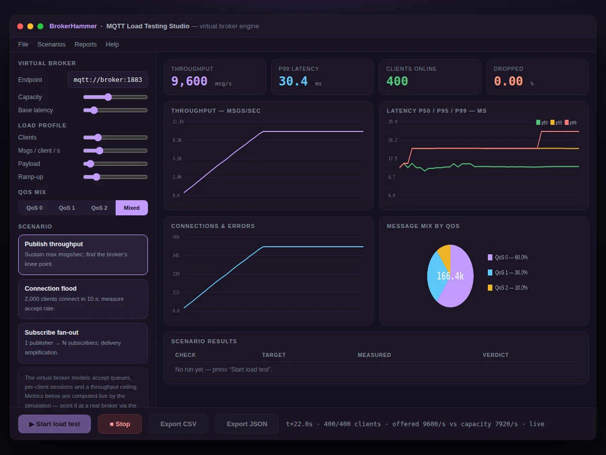
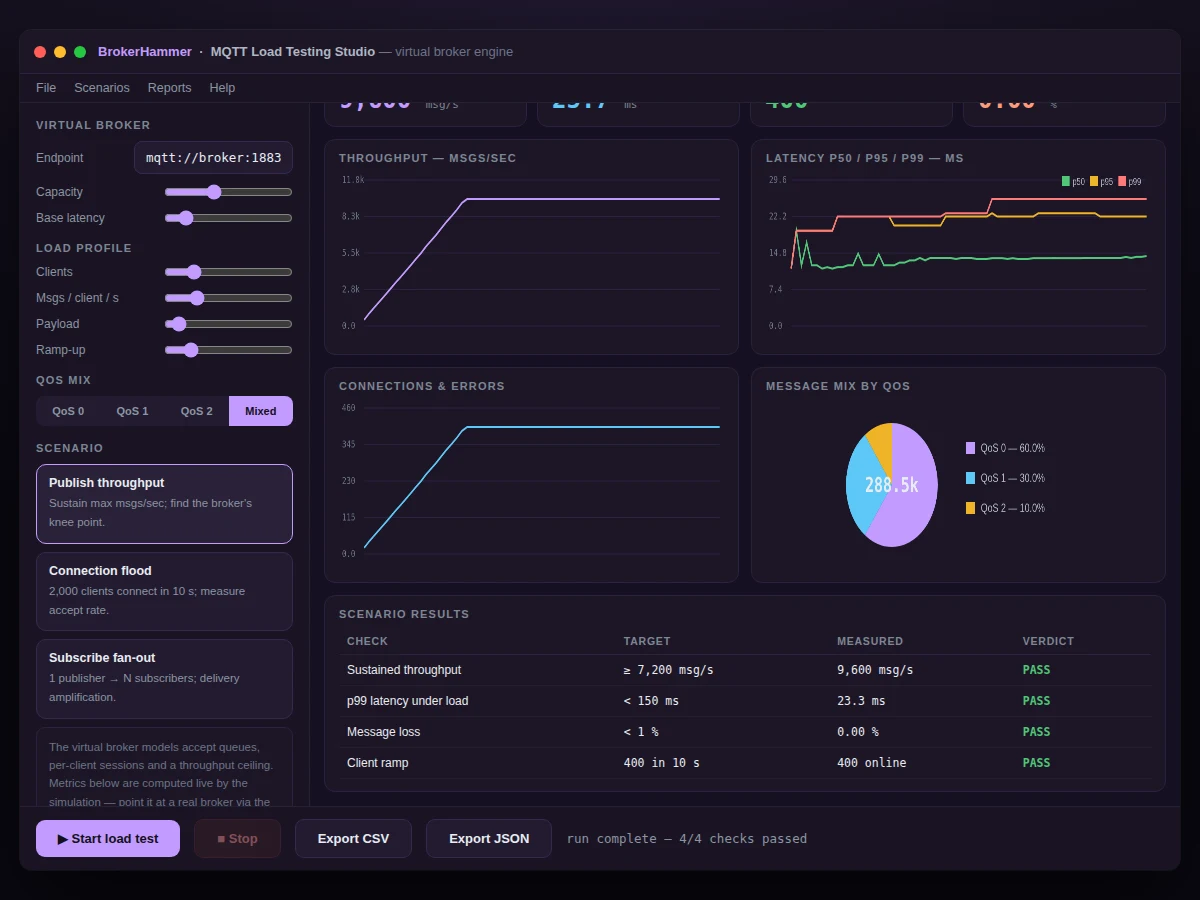
Anyone deploying MQTT at scale — smart-campus sensors, factory telemetry — eventually asks 'how many clients can my broker take before latency explodes?', and answering it against production is risky. This project builds a load-testing studio around a virtual broker engine that models the dynamics honestly: per-client publish rates ramp up over a configurable window, offered load is compared against a throughput ceiling with jitter, latency follows a queueing curve (flat until ~85% load, then climbing), and connection floods inject accept errors. Live canvas charts show throughput, p50/p95/p99 latency, connections and QoS mix; scenario checks (sustained throughput, p99 bound, loss budget, ramp completion) render pass/fail verdicts from measured series; CSV/JSON export carries the full time series for the report. The engine is a teaching model of broker behavior — documented as such — with a bridge API path for hardware-in-the-loop runs against a real broker.
How it works
- The user configures the virtual broker (endpoint label, throughput capacity, base latency) and the load profile (clients, rate, payload, ramp-up, QoS mix).
- On start, virtual clients come online along the ramp curve; each publishes at the configured rate with the selected QoS mix.
- Each 500 ms tick computes offered load (with fan-out amplification in that scenario) against the jittered capacity ceiling; excess is counted as dropped.
- Latency per tick combines base latency, a queueing term that activates above ~85% utilization, and Gaussian jitter; p50/p95/p99 come from a sliding window.
- Charts and KPI cards update live; the run-status line shows clients online, offered vs capacity, and elapsed time.
- On stop (or scenario completion), the verdict engine compares measured sustained throughput, mean p99, loss percentage and ramp completion against targets.
- Export serializes the verdict table and the full time series to CSV or JSON for the report.
Tech stack:
- JavaScript (ES6+)
- Canvas charting (hand-rolled)
- Queueing latency model
- Sliding-window percentiles
- Scenario engine
- CSV/JSON exporters
- Single-file web app
| Parameter | Value |
|---|---|
| Clients | 10–2,000 virtual clients |
| Publish rate | 1–50 msgs/client/s |
| Broker capacity | 1,000–20,000 msgs/s (configurable) |
| Latency model | Base + queueing + jitter; p50/p95/p99 |
| Scenarios | Throughput, flood, fan-out |
| Tick | 500 ms live updates |
| Verdicts | 4 automatic checks vs targets |
| Export | CSV + JSON time series |
Project features
- [Virtual broker engine] Capacity ceiling, base latency, accept queues and per-client sessions modeled live — no real broker needed for the demo.
- [Live metric charts] Canvas-rendered throughput, p50/p95/p99 latency, connections/errors and QoS-mix donut, updating every 500 ms.
- [Load profile controls] Clients (10–2000), msgs/client/s, payload size, ramp-up time, QoS 0/1/2/mixed — all adjustable mid-session.
- [Three test scenarios] Publish throughput (find the knee), connection flood (2,000 connects in 10 s), subscribe fan-out (delivery amplification).
- [Pass/fail verdicts] Sustained throughput, p99 latency bound, loss budget and ramp completion checked against targets automatically.
- [CSV/JSON export] Full time series plus verdict table exported for the project report.
- [Queueing latency model] Latency stays near base until high utilization, then climbs — the classic knee curve, visible live.
What is included
- Single-file load-testing studio (working demo)
- Virtual broker engine source (documented model)
- Scenario definitions (throughput, flood, fan-out)
- User guide: profiles, scenarios, reading verdicts
- Project report PDF (MQTT primer, load-testing theory, queueing model)
- PPT presentation for final review
- Viva Q&A preparation document
Limitations & prerequisites
- The virtual broker is a teaching model of broker dynamics, not a real MQTT implementation — stated in the UI; it cannot replace testing against a real broker, which the bridge API path supports.
- Latency and loss figures are produced by the model, not measured from hardware — the report labels them as simulation outputs.
- MQTT protocol details ( retained messages, wildcards, auth) are out of scope; the engine models load, not protocol conformance.
- The queueing curve parameters are configurable but approximate; real brokers have additional nonlinearities.
- Payload content is synthetic; the engine varies size, not content semantics.
- Browser timing (500 ms ticks) is approximate under heavy tab load.
Frequently Asked Questions
Does this test a real MQTT broker?
The demo runs a virtual broker engine that models throughput ceilings, queueing latency and connection behavior — ideal for learning and demonstrations. The report documents a bridge API path for hardware-in-the-loop runs where the same studio drives a real broker.
What do the p50/p95/p99 latency lines mean?
They are percentiles of per-tick latency samples in a sliding window: p50 is the median, p99 the near-worst case. The gap between p50 and p99 shows how badly tail latency degrades under load — the key broker-sizing signal.
What is the 'knee' in the throughput scenario?
The point where offered load crosses capacity: throughput flattens at the ceiling while latency climbs steeply. The charts make it visible live, and it is the central concept of the viva discussion.
How are pass/fail verdicts decided?
Four checks compare measured series against targets: sustained throughput ≥ 90% of capacity, mean p99 < 150 ms, loss < 1%, and ramp completion ≥ 98% of clients. Targets are adjustable in the verdict engine.
Can I export results for my report?
Yes — CSV and JSON exports carry the verdict table plus the full time series (throughput, percentiles, clients) for plotting in the report.
Is this project suitable for a final-year project?
Yes — for Computer Science and IT programs. It covers MQTT and pub/sub messaging, performance testing methodology, queueing theory and live data visualization. Suitable for B.E./B.Tech final-year projects in Computer Science and IT.
Components & software requirements
- JavaScript (ES6+)
- Canvas charting (hand-rolled)
- Queueing latency model
- Sliding-window percentiles
- Scenario engine
- CSV/JSON exporters
- Single-file web app
Delivery information
Built-to-order project. Delivery timeline is shared after order confirmation based on current queue.
Support terms
Complete documentation, setup guide, and viva preparation included. Support for setup and explanation provided.