
More project photos (2)
The problem
Everyone who plans electricity supply — from grid operators balancing load to households choosing a tariff — needs to know how much energy will be used tomorrow, next week and next season. Classical methods like ARIMA demand statistical expertise, stationarity assumptions and manual tuning, and they struggle when a series carries several overlapping rhythms at once: a household uses power differently at 7 AM versus 7 PM, on weekdays versus weekends, and in January versus July. This project applies Prophet to the UCI Individual Household Electric Power Consumption dataset (over 2 million minute-level readings from a French household, December 2006–November 2010): ingestion and resampling, Prophet modeling with daily/weekly/yearly seasonality and holiday effects, changepoint tuning, forecast horizons with uncertainty intervals, holdout backtesting with MAPE/RMSE/MAE, seasonality decomposition, and a dashboard demo with adjustable horizon.
How it works
- The UCI household power dataset (2,074,259 minute-level records, December 2006–November 2010) is ingested, gap-checked and resampled to an hourly or daily consumption series.
- A Prophet model is specified with daily, weekly and yearly seasonality (Fourier terms), French public-holiday effects, and automatic changepoint detection on the trend.
- The model is fitted on the training history; changepoint prior scale is tuned by comparing fits, documented in the notebook.
- Forecasts are generated for the chosen horizon with uncertainty intervals that widen as the horizon extends.
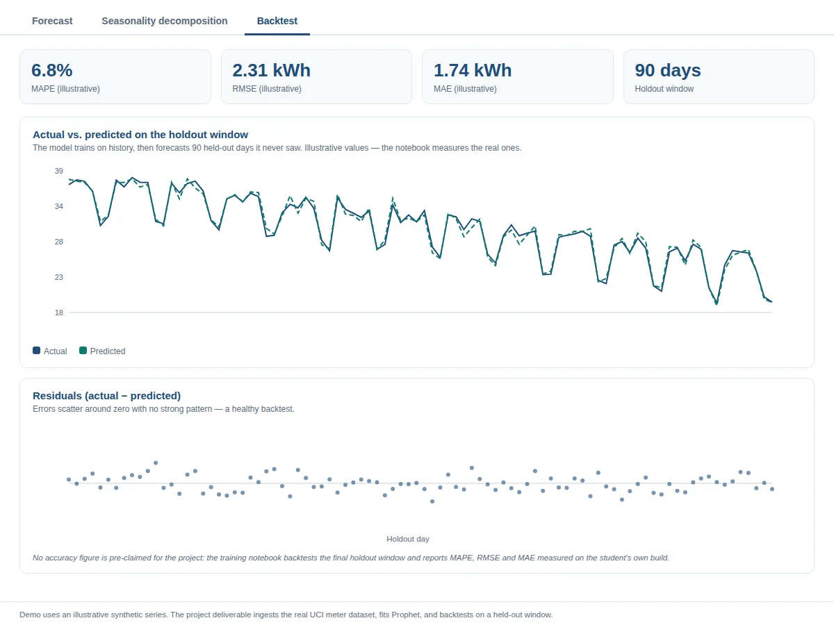
- A final holdout window (e.g. the last 90 days) is backtested: MAPE, RMSE and MAE are computed and actual-vs-predicted plotted.
- The demo renders history plus forecast, the decomposed seasonality components, and the backtest panel with an adjustable horizon control.
Tech stack:
- Python 3.10, Prophet (additive forecasting: trend, seasonality, holidays)
- pandas, NumPy (resampling and series wrangling)
- Matplotlib, Seaborn (forecast bands, decomposition, backtest plots)
- scikit-learn (MAPE/RMSE/MAE metrics)
- Jupyter notebook (buyer-run training and evaluation)
- Streamlit demo app (forecast dashboard, decomposition viewer, backtest panel)
| Parameter | Value |
|---|---|
| Model | Facebook Prophet — additive y(t) = trend + seasonality + holidays + error |
| Dataset | UCI Individual Household Electric Power Consumption — 2,074,259 minute-level readings, Dec 2006–Nov 2010 |
| Seasonality | Daily, weekly and yearly Fourier components plus French holiday effects |
| Trend | Piecewise-linear with automatic changepoint detection (tunable prior scale) |
| Evaluation | MAPE, RMSE, MAE on a held-out window with actual-vs-predicted overlay — computed on your build by the notebook |
| Output | Forecasted kWh per period with uncertainty intervals; decomposed components; peak-demand days |
| Horizons | 7 / 30 / 90-day forecasts from the demo's horizon control |
| Inference | Batch forecast generation in the notebook; interactive dashboard in the demo app |
Project features
- [UCI meter-data pipeline] Ingests the Individual Household Electric Power Consumption dataset (2,074,259 minute-level records), handles gaps and resamples to hourly or daily series for modeling.
- [Prophet additive model] Fits trend plus daily, weekly and yearly seasonality with Fourier terms, French holiday effects, and automatic changepoint detection for trend shifts.
- [Changepoint sensitivity tuning] Exposes the changepoint prior scale so the report can compare stiff versus flexible trend fits on the same data.
- [Forecast horizon control] Generates 7, 30 or 90-day forecasts with Prophet's uncertainty intervals, visualized as widening bands the further ahead the forecast reaches.
- [Holdout backtesting] Trains on history, forecasts a held-out window, and reports MAPE, RMSE and MAE with an actual-vs-predicted overlay — all computed by the notebook during the build.
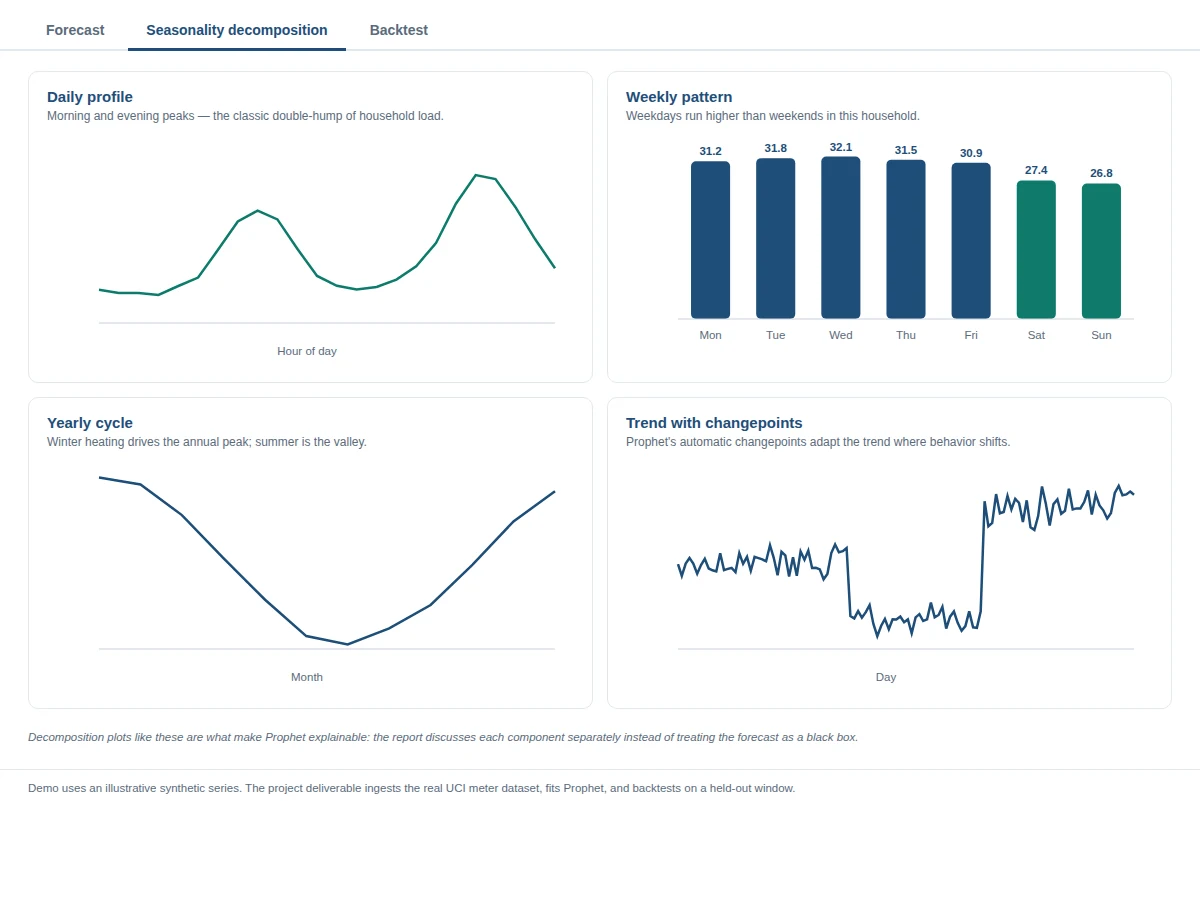
- [Seasonality decomposition viewer] Plots the separated trend, daily profile, weekly pattern and yearly cycle components so the report can explain what the model learned.
- [Peak-demand analysis] Identifies the highest-load days in history and in the forecast, the figures a utility planner actually cares about.
- [Scenario comparison] Compares a normal week's forecast against a holiday week's, showing how the holiday component shifts predicted consumption.
What is included
- Complete source code (data pipeline, Prophet modeling, backtesting, demo app)
- Jupyter training and evaluation notebook (buyer-run procedure from ingestion to forecast)
- Project report PDF (background, Prophet theory, methodology, decomposition analysis, backtest results)
- PPT presentation for final review
- Viva Q&A preparation document (Prophet internals, Fourier seasonality, changepoints, MAPE vs RMSE, stationarity)
- Setup guide (environment, dataset download, running the notebook and demo)
Limitations & prerequisites
- The data is a single French household from 2006–2010; it does not represent other climates, household sizes, or today's appliance mix — this is a teaching benchmark, not a utility planning tool.
- Weather, the strongest short-term driver of heating and cooling load, is not in the feature set; the report notes this as the main accuracy lever left unused.
- Prophet assumes repeating seasonal patterns and misses one-off events (heatwaves, lockdowns, equipment failures) that break the rhythm.
- Minute-level noise is smoothed away by resampling; the model forecasts aggregate consumption, not appliance-level disaggregation.
- There is no real-time smart-meter integration in the base build; forecasts run on the historical dataset in batch.
Frequently Asked Questions
Which dataset is used?
The UCI Individual Household Electric Power Consumption dataset: 2,074,259 minute-level readings (global active/reactive power, voltage, current, sub-meterings) from one household in Sceaux, France, spanning December 2006 to November 2010. It is freely available from the UCI Machine Learning Repository.
Why Prophet instead of ARIMA or LSTM?
Household load carries daily, weekly and yearly rhythms plus holiday effects and trend shifts — Prophet models each component explicitly with Fourier seasonality and automatic changepoints, tolerates missing readings, and needs no stationarity preprocessing, while remaining explainable through its decomposition plots.
Is the forecast accuracy guaranteed?
No. The notebook backtests the final holdout window and reports MAPE, RMSE and MAE — those measured values are the report's numbers, not a promise. Accuracy depends on the resampling grain, horizon length and how stable the household's routines are.
How does Prophet handle the different seasonalities?
Each seasonality is a sum of Fourier sine/cosine terms at the appropriate period (24 hours, 7 days, 365.25 days); Prophet fits their coefficients jointly with the trend, and the demo's decomposition viewer plots each component separately.
Can it forecast for another household or country?
Yes, with retraining: any timestamped consumption series works. Swap in the new data, re-specify the holiday calendar for the country, refit in the notebook, and the dashboard renders the new forecast unchanged.
What will the project report analyze?
The decomposed trend and seasonal components (what the model learned about daily/weekly/yearly rhythms), the changepoint tuning comparison, the backtest error metrics with the actual-vs-predicted overlay, and the peak-demand findings.
Suitable for B.E./B.Tech final-year projects in Computer Science, AI/ML and Data Science.
Components & software requirements
- Python 3.10, Prophet (additive forecasting: trend, seasonality, holidays)
- pandas, NumPy (resampling and series wrangling)
- Matplotlib, Seaborn (forecast bands, decomposition, backtest plots)
- scikit-learn (MAPE/RMSE/MAE metrics)
- Jupyter notebook (buyer-run training and evaluation)
- Streamlit demo app (forecast dashboard, decomposition viewer, backtest panel)
Delivery information
Built-to-order project. Delivery timeline is shared after order confirmation based on current queue.
Support terms
Complete documentation, setup guide, and viva preparation included. Support for setup and explanation provided.