
More project photos (2)
The problem
Keyword search fails the moment images have no reliable tags — personal photo libraries, surveillance archives and product catalogues all hold millions of untagged pictures. Content-based image retrieval (CBIR) solves this by describing each image with numbers computed from its own pixels and ranking the collection by visual similarity to a query image. This project implements the classical, fully transparent CBIR pipeline end to end: every image is reduced to a 2×2 spatial RGB histogram (256 dimensions) plus Sobel edge density (1 dimension), the vectors are L2-normalized and indexed, and a query is answered by chi-squared distance ranking. A live web demo makes the engine tangible — pick any photo as the query and the app shows the ranked results with similarity scores, while a feature inspector reveals the exact 257-dimensional vector the engine computed. Because every stage is classical and inspectable, the student can explain precisely why each result was returned.
How it works
- Each collection image is divided into a 2×2 spatial grid; a 64-bin RGB histogram is computed per cell and concatenated into a 256-D vector.
- Sobel edge density (fraction of edge pixels) is appended, forming the final 257-D descriptor, which is L2-normalized and stored in the index.
- A query image goes through the identical extraction, guaranteeing query and index vectors live in the same space.
- Chi-squared distance is computed between the query vector and every indexed vector; the collection is ranked by ascending distance and the top-K returned.
- The evaluation harness replays every benchmark image as a query, marks same-category hits as relevant, and computes Precision@K and mAP.
- The fused variant concatenates the 257-D classical vector with a 2048-D CNN embedding before ranking, and the harness measures the improvement.
Tech stack:
- Python 3, NumPy, OpenCV (feature extraction)
- scikit-learn (metrics)
- Jupyter Notebook (evaluation harness)
- Flask/FastAPI (REST query API)
- HTML5 + JavaScript (live retrieval demo)
- Wang image database (Corel-1K)
Dataset & model details
- Dataset: Wang image database (Corel-1K, James Z. Wang, Penn State) — 1,000 photographs in 10 categories × 100 images (African people, beaches, buildings, buses, dinosaurs, elephants, flowers, horses, mountains, food). Ground truth: same-category images count as relevant for a query.
- Task: Query-by-example retrieval; input = a query image, output = the collection ranked by visual similarity (top-K list with similarity scores).
- Model: Classical: 257-D descriptor (2×2 spatial RGB histogram + Sobel edge density), L2-normalized, chi-squared distance ranking. Fused variant: 257-D classical concatenated with a 2048-D CNN embedding, cosine/chi-squared ranking.
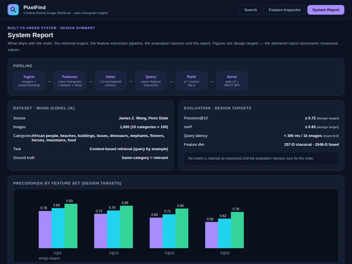
- Metrics: Precision@10 ≥ 0.72 (design target), mAP ≥ 0.65 (design target), Precision@K curves for K = 5/10/20/50, query latency < 300 ms per 1,000 images (expected). No metric is claimed as measured until the evaluation harness runs for the order.
| Parameter | Value |
|---|---|
| Feature vector | 257-D classical (256 histogram + 1 edge) · 2048-D fused |
| Distance metric | Chi-squared (histograms) / cosine (fused) |
| Benchmark | Wang (Corel-1K): 1,000 images, 10 categories |
| Precision@10 | ≥ 0.72 (design target, not a measured claim) |
| mAP | ≥ 0.65 (design target) |
| Query latency | < 300 ms per 1,000 images (expected) |
| Index | L2-normalized vectors, in-memory |
| Demo | Single-file web app, runs offline after download |
Project features
- [Real histogram-matching engine] 2×2 spatial RGB histograms plus Sobel edge density extracted live from actual pixels — 257-D vectors, L2-normalized, ranked by chi-squared distance. No tags, no filenames, pure visual similarity.
- [Live retrieval demo] Pick any photo as the query; the engine extracts its features and returns the collection ranked most-similar-first with similarity scores and rank badges.
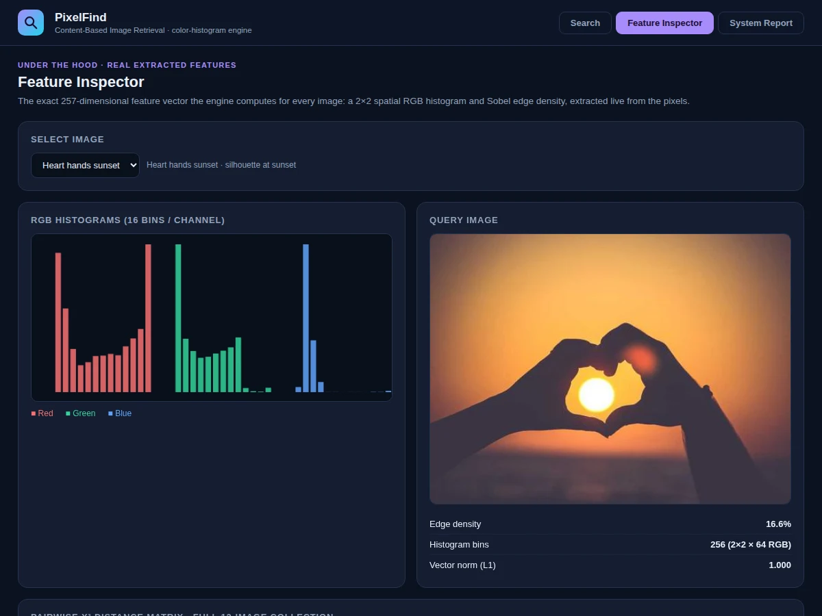
- [Feature inspector] Select any image to see its exact RGB histograms (16 bins/channel), edge density and vector norm — the full internals of the engine, exposed.
- [Pairwise distance matrix] The complete chi-squared distance matrix over the demo collection, showing how the metric separates similar from dissimilar images.
- [Evaluation harness] Precision@K and mean average precision computed on the Wang (Corel-1K) benchmark with same-category ground truth, in a reproducible notebook.
- [Deep-fusion variant] The classical 257-D descriptor concatenated with a 2048-D CNN embedding for a fused representation, with the measured gain documented.
- [Web UI + REST API] The retrieval engine served behind a clean web interface and a query API, as the pipeline diagram in the demo shows.
What is included
- Complete CBIR engine (ingest, feature extraction, indexing, ranking, serving)
- Evaluation harness notebook with Precision@K and mAP on Corel-1K
- Live retrieval + feature inspector + system report web demo
- Pairwise distance matrix and precision@K-by-feature-set charts
- Project report PDF (retrieval theory, histogram methods, distance metrics, methodology, results)
- PPT presentation for final review
- Viva Q&A preparation document (color spaces, histograms, chi-squared, precision/recall in retrieval)
Limitations & prerequisites
- Color histograms ignore spatial layout within each grid cell and object semantics — a red car and a red apple can rank as similar; the report discusses this honestly.
- Precision@10 ≥ 0.72 and mAP ≥ 0.65 are design targets for the evaluation run, stated honestly — the report documents the actual measured figures after the harness runs.
- The demo collection is a small curated set for interactivity; the full 1,000-image benchmark runs in the evaluation notebook, not in the browser.
- The fused CNN variant improves semantic matching but adds inference cost — the tradeoff is measured and reported.
- Retrieval quality depends on the collection: near-duplicate or very dark images compress the distance range.
Frequently Asked Questions
How does it find similar images without tags?
Each image is converted to a 257-dimensional numeric description (spatial color histogram + edge density) computed from its pixels. Similarity is then pure arithmetic — the chi-squared distance between the query's vector and every stored vector.
Why chi-squared distance instead of Euclidean?
Chi-squared is the standard metric for comparing histograms: it normalizes each bin's contribution by the bin magnitudes, so large bins don't drown out small but informative ones. The report derives this choice.
What is the Wang (Corel-1K) dataset?
A 1,000-image benchmark from James Z. Wang's group at Penn State: 10 everyday categories with 100 photos each. Same-category images serve as ground-truth relevant results, making precision measurable.
What does the fused variant add?
Concatenating the 257-D classical descriptor with a 2048-D CNN embedding adds semantic understanding (objects, scenes) that pure color statistics miss. The harness quantifies the Precision@K gain of fusion over classical alone.
Can it search my own photo collection?
Yes — the ingest stage indexes any folder of images into the same vector format, and the REST API answers queries over it. Indexing your own collection is documented as an extension.
Is this project suitable for a final-year project?
Yes — for AI/ML, Computer Science and IT programs. It demonstrates feature engineering, distance metrics, information-retrieval evaluation and a working live search demo. Suitable for B.E./B.Tech final-year projects in AI & Machine Learning, Computer Science and IT.
Components & software requirements
- Python 3, NumPy, OpenCV (feature extraction)
- scikit-learn (metrics)
- Jupyter Notebook (evaluation harness)
- Flask/FastAPI (REST query API)
- HTML5 + JavaScript (live retrieval demo)
- Wang image database (Corel-1K)
Dataset & model details
- Dataset: Wang image database (Corel-1K, James Z. Wang, Penn State) — 1,000 photographs in 10 categories × 100 images (African people, beaches, buildings, buses, dinosaurs, elephants, flowers, horses, mountains, food). Ground truth: same-category images count as relevant for a query.
- Task: Query-by-example retrieval; input = a query image, output = the collection ranked by visual similarity (top-K list with similarity scores).
- Model: Classical: 257-D descriptor (2×2 spatial RGB histogram + Sobel edge density), L2-normalized, chi-squared distance ranking. Fused variant: 257-D classical concatenated with a 2048-D CNN embedding, cosine/chi-squared ranking.
- Metrics: Precision@10 ≥ 0.72 (design target), mAP ≥ 0.65 (design target), Precision@K curves for K = 5/10/20/50, query latency < 300 ms per 1,000 images (expected). No metric is claimed as measured until the evaluation harness runs for the order.
Delivery information
Built-to-order project. Delivery timeline is shared after order confirmation based on current queue.
Support terms
Complete documentation, setup guide, and viva preparation included. Support for setup and explanation provided.