
More project photos (2)
The problem
Breast cancer diagnosis rests on the pathologist's microscope: H&E-stained tissue slides are examined at multiple magnifications for the architectural and nuclear changes that separate benign from malignant tissue. It is skilled, time-consuming work, and pathologist workloads keep growing — which is why automated histopathology analysis is one of the most published areas in medical computer vision. The BreaKHis dataset (Spanhol et al., 2016) — 7,909 microscopy images from 82 patients, labeled benign or malignant across 8 subtypes and 4 magnifications — is the standard academic benchmark for the task. This project builds the canonical student solution: a transfer-learned patch classifier with stain normalization, strict patient-wise splitting (the leakage trap examiners ask about first), per-magnification evaluation and a demo that visualizes what benign vs malignant tissue looks like. It is designed as a rigorous classification build while being explicit that it is a research prototype — histopathology diagnosis stays with the pathologist.
How it works
- BreaKHis images are loaded (7,909 H&E patches, 700x460 px, benign vs malignant labels with 8 subtype labels and 4 magnification levels) and grouped by patient ID.
- Patients are split into train/validation/test sets; patches inherit their patient's split, guaranteeing no leakage between sets.
- H&E stain normalization is applied, patches are resized to 224x224 and augmented with rotations, flips and color jitter appropriate for microscopy.
- An ImageNet-pretrained ResNet50 (or EfficientNet-B0) is fine-tuned with a binary head, logging loss, accuracy and AUC per epoch on the validation patients.
- The evaluation notebook computes final metrics on held-out patients — accuracy, AUC, sensitivity, specificity, confusion matrix — broken down per magnification level and per subtype.
- The Flask demo classifies an uploaded patch, shows the benign/malignant probabilities with the nuclei-highlight overlay, and labels the output as a research aid.
Tech stack:
- Python 3.10, PyTorch with timm (ResNet50 / EfficientNet-B0 transfer learning)
- OpenCV, scikit-image (patch extraction, stain normalization)
- scikit-learn (metrics, ROC-AUC, patient-wise splits)
- Matplotlib, Seaborn (curves, ROC plots, confusion matrix)
- Flask demo web app (patch upload, comparison viewer, nuclei overlay)
- Jupyter notebook (buyer-run training and evaluation)
| Parameter | Value |
|---|---|
| Task | Binary histopathology patch classification (benign vs malignant) |
| Dataset | BreaKHis (Spanhol et al., 2016) — 7,909 H&E images, 82 patients, P&D Lab Brazil |
| Classes | Benign (2,480: adenosis, fibroadenoma, phyllodes tumor, tubular adenoma) / Malignant (5,429: ductal, lobular, mucinous, papillary carcinoma) |
| Magnifications | 40x, 100x, 200x, 400x (700x460 px RGB PNG) |
| Model | ResNet50 / EfficientNet-B0, ImageNet transfer learning, binary head, stain normalization |
| Input | H&E patches resized to 224x224 |
| Output | Benign/malignant probabilities, nuclei-highlight overlay |
| Evaluation | Accuracy, AUC, sensitivity, specificity, confusion matrix — per magnification and per subtype, computed by the notebook on held-out patients |
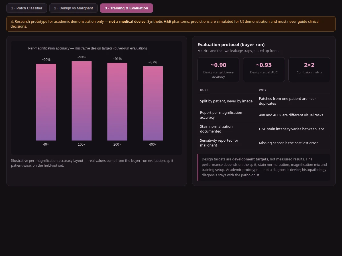
| Design targets | Binary accuracy ~0.90, AUC ~0.93 (targets, not measured claims) |
| Demo | Flask app with upload, benign-vs-malignant comparison viewer |
| Scope note | Academic research prototype — not a medical device; histopathology diagnosis stays with the pathologist |
Project features
- [Binary patch classifier] ResNet50 / EfficientNet-B0 fine-tuned on BreaKHis patches for benign vs malignant classification, with the 8-subtype experiment documented as an extension.
- [Patient-wise split enforcement] Splitting by patient ID (82 patients), never by image — patches from one patient are near-duplicates, and the notebook verifies the split is leak-free.
- [Stain normalization] Macenko-style H&E stain normalization in preprocessing, with a documented comparison of with/without normalization since stain intensity varies between labs.
- [Multi-magnification training] The model trains on the mixed 40x/100x/200x/400x set and the notebook reports per-magnification accuracy, showing which zoom levels are hardest.
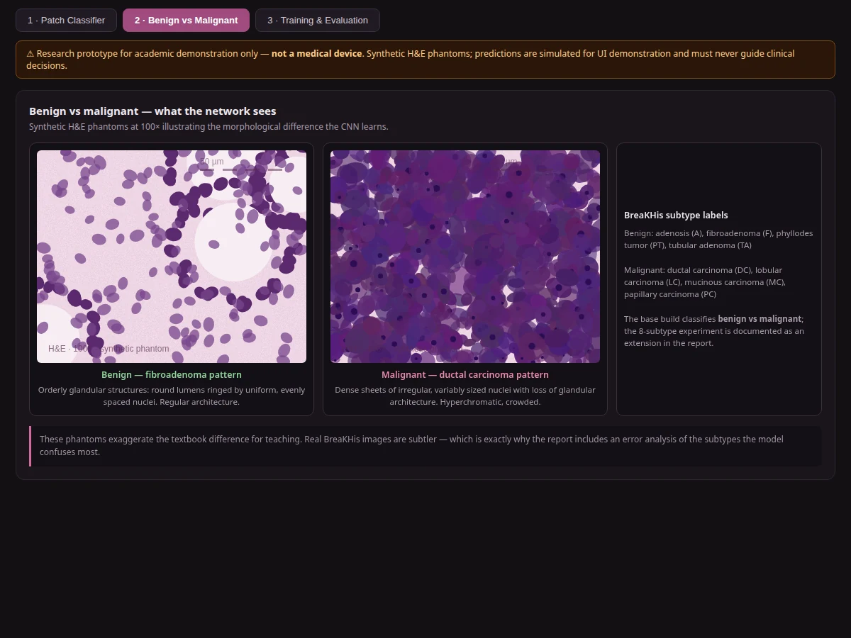
- [Nuclei-highlight viewer] The demo can overlay detected nuclei contours on the patch, visualizing the nuclear crowding and irregularity the network keys on.
- [Subtype error analysis] Confusion analysis across the 8 BreaKHis subtypes (adenosis, fibroadenoma, phyllodes, tubular adenoma; ductal, lobular, mucinous, papillary carcinoma) for honest viva material.
- [Patch extraction pipeline] Whole-image to patch utilities with configurable patch size and stride, plus background filtering so empty slide regions don't pollute training.
- [Comparison demo mode] Side-by-side benign vs malignant patch viewer with magnification switching, built for classroom and viva demonstration.
What is included
- Complete source code (patch pipeline, stain normalization, training, demo app, evaluation utilities)
- Jupyter training and evaluation notebook (buyer-run: patient-wise splits, train, per-magnification evaluation, subtype analysis)
- Flask demo application with patch upload and comparison viewer
- Project report PDF (background, BreaKHis analysis, leakage-safe methodology, evaluation, subtype error analysis, limitations)
- PPT presentation for final review
- Viva Q&A preparation document (transfer learning, patient-wise splitting, stain normalization, AUC, H&E imaging)
- Setup guide (environment, dataset download, training on CPU/GPU, running the demo)
Limitations & prerequisites
- This is an academic prototype, not a medical device: not clinically validated, not certified, and must never guide diagnosis or treatment — histopathology diagnosis stays with the pathologist.
- BreaKHis comes from a single lab's 82 patients, so stain characteristics, scanner and population are narrow; performance on other labs' slides is not promised and stain normalization only partly bridges the gap.
- The base build classifies benign vs malignant only; the finer 8-subtype task is harder and is documented as an extension, not a solved problem.
- Patch-level predictions are not whole-slide diagnosis — real pathology reads the entire slide in context, which this project does not attempt.
- Class imbalance (5,429 malignant vs 2,480 benign) and the small patient count keep minority-subtype metrics noisy; the report states this openly.
- Reported metrics come from the buyer's own training run and vary with patient split, stain normalization and hyperparameters; design targets are goals, not guarantees.
Frequently Asked Questions
Which dataset is used?
BreaKHis (Breast Cancer Histopathological Image Database, Spanhol et al., 2016): 7,909 H&E-stained microscopy images from 82 patients, labeled benign vs malignant across 8 subtypes and 4 magnification levels (40x–400x).
Why must the split be by patient, not by image?
Patches from the same patient look nearly identical — an image-wise split leaks near-duplicates into the test set and inflates accuracy. The notebook splits by patient ID and verifies the split, which is the methodologically correct approach.
Is the accuracy guaranteed?
No. The page states design targets (binary accuracy ~0.90, AUC ~0.93), but actual numbers come from your training run on your held-out patients — reported per magnification and per subtype — and the report presents those.
Is this a medical device? Can it diagnose breast cancer?
No. This is strictly an academic research prototype for learning histopathology image classification. It is not clinically validated or certified and must never be used to assess real tissue — diagnosis stays with the pathologist.
What is stain normalization and why does it matter?
H&E stain intensity varies between labs and batches, shifting image colors. Stain normalization standardizes colors before training so the model learns tissue morphology rather than one lab's staining style; the notebook compares with/without it.
What will I receive with the project?
Source code, the training/evaluation notebook, the Flask demo app, report PDF, PPT, viva Q&A document and setup guide — everything prepared fresh for your build. Suitable for B.E./B.Tech final-year projects in Computer Science, AI/ML and Data Science.
Components & software requirements
- Python 3.10, PyTorch with timm (ResNet50 / EfficientNet-B0 transfer learning)
- OpenCV, scikit-image (patch extraction, stain normalization)
- scikit-learn (metrics, ROC-AUC, patient-wise splits)
- Matplotlib, Seaborn (curves, ROC plots, confusion matrix)
- Flask demo web app (patch upload, comparison viewer, nuclei overlay)
- Jupyter notebook (buyer-run training and evaluation)
Delivery information
Built-to-order project. Delivery timeline is shared after order confirmation based on current queue.
Support terms
Complete documentation, setup guide, and viva preparation included. Support for setup and explanation provided.