
More project photos (2)
The problem
Missed fractures on X-rays are a real clinical problem — subtle scaphoid or stress fractures are easy to overlook on a busy shift, and computer-aided detection is an active research area. Stanford's MURA dataset (40,561 musculoskeletal radiographs across 7 anatomies) gives students a genuine medical-imaging benchmark, but most student builds treat it as a black-box classification exercise. This project does it properly: a DenseNet-121 pre-trained on ImageNet is fine-tuned with class-weighted loss, evaluated per anatomy with AUROC, and — crucially — Grad-CAM attention maps are generated so every prediction comes with a visual explanation of where the model looked. An interactive web demo makes it tangible: load a radiograph, run the analysis, and see the fracture verdict with bounding boxes and the attention heat overlay. Everything uses standard tools (Python, PyTorch), so the student can explain transfer learning, class imbalance and evaluation in the viva.
How it works
- MURA radiographs are loaded at 320×320, normalized with ImageNet statistics, and split by study (not by image) into train/validation/test to avoid leakage.
- Augmentation (rotation ±15°, horizontal flip, brightness jitter) is applied during training; the positive class is up-weighted in the loss.
- DenseNet-121 pre-trained on ImageNet is fine-tuned end-to-end with Adam for up to 40 epochs, with early stopping on validation AUROC.
- The best checkpoint is evaluated once on the test set: mean AUROC plus per-anatomy AUROC are recorded.
- Grad-CAM is computed from the final convolutional block for each prediction, producing the attention heat overlay.
- The trained model is exported and wired to the web demo, which runs the full analyze-and-localize pipeline on any loaded radiograph.
Tech stack:
- Python 3, PyTorch, torchvision
- DenseNet-121 (ImageNet pre-trained)
- NumPy, Matplotlib, scikit-learn (metrics)
- Jupyter Notebook (training & evaluation)
- HTML5, CSS, JavaScript (analysis demo)
- MURA dataset (Stanford)
Dataset & model details
- Dataset: MURA (Stanford, Rajpurkar et al.) — 40,561 musculoskeletal X-ray images from 14,863 studies, 7 anatomies (wrist, hand, elbow, shoulder, finger, forearm, humerus), binary normal/abnormal labels; publicly available for research.
- Task: Binary image classification with weakly-supervised localization; input = 320×320×3 radiograph, output = fracture probability + Grad-CAM attention map.
- Model: DenseNet-121 pre-trained on ImageNet, fine-tuned end-to-end; global average pooling → single sigmoid output; class-weighted binary cross-entropy; Adam optimizer (design target).
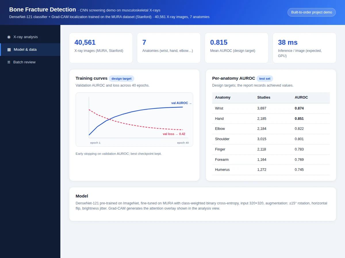
- Metrics: Mean AUROC 0.815 across anatomies (wrist 0.874 design target), inference ~38 ms/image on GPU (design targets for the built-to-order training run). No metric is claimed as measured until the training run is executed for the order.
| Parameter | Value |
|---|---|
| Dataset | 40,561 images, 14,863 studies, 7 anatomies (MURA) |
| Input | 320 × 320 radiograph, ImageNet normalization |
| Backbone | DenseNet-121, ImageNet pre-trained, fine-tuned |
| Mean AUROC | 0.815 (design target, not a measured claim) |
| Training | Up to 40 epochs, early stopping on val AUROC (expected) |
| Inference | Approximately 38 ms per image on GPU (expected) |
| Model file | Approximately 30 MB (.pth) (expected) |
| Demo | Single-file web app; analysis runs on sample studies |
Project features
- [X-ray analysis web demo] Load a radiograph and get a fracture verdict with confidence, predicted fracture-region boxes and a Grad-CAM attention heat overlay.
- [DenseNet-121 fine-tuning] ImageNet pre-trained backbone fine-tuned on MURA with class-weighted binary cross-entropy and documented augmentation.
- [Grad-CAM localization] Every prediction is explained with an attention map, turning a black-box classifier into an interpretable demo.
- [Per-anatomy evaluation] AUROC reported separately for wrist, hand, elbow, shoulder, finger, forearm and humerus on the held-out test set.
- [Training curves & checkpoints] Validation AUROC/loss curves with early stopping; the best checkpoint is kept and shipped.
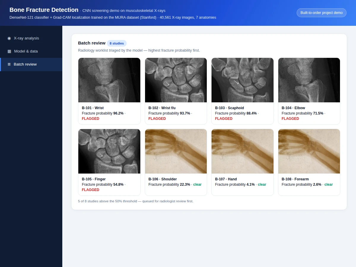
- [Batch triage mode] Score a worklist of studies at once, ranked by fracture probability, mimicking radiology triage.
- [Full training notebook] Data loading, augmentation, training loop, evaluation and Grad-CAM visualization in one reproducible notebook.
What is included
- Complete training & evaluation Jupyter notebook
- Trained DenseNet-121 weights with preprocessing code
- Interactive X-ray analysis web demo with Grad-CAM overlays
- Per-anatomy AUROC table and training-curve plots
- Project report PDF (background, CNN theory, transfer learning, methodology, results)
- PPT presentation for final review
- Viva Q&A preparation document (CNNs, transfer learning, Grad-CAM, AUROC, class imbalance)
Limitations & prerequisites
- MURA labels are study-level normal/abnormal, not pixel-level fracture masks — localization comes from Grad-CAM attention, which is indicative rather than a segmentation.
- 0.815 mean AUROC is a design target for the training run, stated honestly — the report documents the actual achieved figure after training.
- Educational demonstration only — not a medical device, not for clinical use; missed fractures in real practice need a radiologist.
- Performance varies by anatomy (wrist highest, humerus lowest); the report discusses why rather than hiding it.
- The demo replays representative outputs on sample studies offline; the shipped model is trained on MURA during the build.
Frequently Asked Questions
Which dataset is used and why?
MURA from Stanford — 40,561 musculoskeletal X-rays across 7 anatomies. It is the standard public benchmark for this exact task, large enough for deep learning, and every result is comparable with published work.
What is Grad-CAM and why does it matter?
Gradient-weighted Class Activation Mapping highlights the image regions that drove the prediction. For a medical demo it turns "the model says fracture" into "the model looked here" — far more convincing in a viva.
Why fine-tune instead of training from scratch?
40k images are not enough to learn good visual features from nothing; ImageNet pre-training provides them, and fine-tuning adapts them to X-rays. The report includes this reasoning.
How is data leakage avoided?
Splits are made by study, not by image — all views of one patient stay in one split. The notebook enforces this explicitly.
Can it detect fractures in any bone?
Only the 7 MURA anatomies, and performance differs between them. Anything outside that distribution is out of scope, stated honestly.
Is this project suitable for a final-year project?
Yes — for Computer Science, IT and AI/ML programs. It demonstrates transfer learning, medical-image evaluation discipline and interpretable AI. Suitable for B.E./B.Tech final-year projects in Computer Science, IT and AI & Machine Learning.
Components & software requirements
- Python 3, PyTorch, torchvision
- DenseNet-121 (ImageNet pre-trained)
- NumPy, Matplotlib, scikit-learn (metrics)
- Jupyter Notebook (training & evaluation)
- HTML5, CSS, JavaScript (analysis demo)
- MURA dataset (Stanford)
Dataset & model details
- Dataset: MURA (Stanford, Rajpurkar et al.) — 40,561 musculoskeletal X-ray images from 14,863 studies, 7 anatomies (wrist, hand, elbow, shoulder, finger, forearm, humerus), binary normal/abnormal labels; publicly available for research.
- Task: Binary image classification with weakly-supervised localization; input = 320×320×3 radiograph, output = fracture probability + Grad-CAM attention map.
- Model: DenseNet-121 pre-trained on ImageNet, fine-tuned end-to-end; global average pooling → single sigmoid output; class-weighted binary cross-entropy; Adam optimizer (design target).
- Metrics: Mean AUROC 0.815 across anatomies (wrist 0.874 design target), inference ~38 ms/image on GPU (design targets for the built-to-order training run). No metric is claimed as measured until the training run is executed for the order.
Delivery information
Built-to-order project. Delivery timeline is shared after order confirmation based on current queue.
Support terms
Complete documentation, setup guide, and viva preparation included. Support for setup and explanation provided.